Figure 29.1 Though MR scanners are primarily used to make images of humans for medical diagnoses, they can also produce exquisite images of the complex tissue water structures within vegetables and fruit. Shown here clockwise from top left are a potato, a pomegranate, a cup of water with ice cube, and a coconut. The absence of signal from the seeds of the pomegranate and the ice cube are due to their solid nature, not to a lack of protons. The dark void in the cup of water from the ice cube may seem surprising since ice is water with a slightly lower PD (that’s why ice floats) … but not that much! The void in the coconut is in fact due to a lack of water protons within the air there. The far right column depicts the organizing principle of the book chapter.

But back to Pink Floyd’s “Us and Them.” Namely, what is it that we (Us) do, and what is it that they (Them) do that together yields the medical miracle of MRI? The following two sections will be dedicated to “Us” and “Them,” respectively, describing what it is that we do to make MR images and what it is that they do to deliver the rich soft tissue contrast achievable from MRI. The final “Us and Them” section emphasizes the interplay between our many and varied pulse sequences and associated machinations which we use to manipulate the water and fat signals to our advantage in making accurate and comprehensive diagnostic assessments.

“Us”

Images are initially composed of “signals” collected by Us and converted into MR images for interpretation. What are these “signals”? In MRI the term “signal” is effectively identical to the term “signal” as used in discussing your favorite radio station. It is a time varying voltage originally in the radio-frequency (RF) range, e.g., the megahertz (MHz) range which, as in FM radio, is converted down to the kilohertz (kHz) range using a reference MHz frequency for convenient listening. Unlike your favorite radio station, however, where the signal comes from broadcasting antennae, the MR signal comes from protons of the hydrogen atoms in the water and lipids of whatever sample has been placed in the magnet. Obtaining this signal requires several basic hardware components, some recognized early in the history (circa 1940s) of nuclear MR (NMR) and some added to accommodate its extension to MRI in the late 1970s. There is first and foremost the great big magnet complete with the whole-body accommodating, and somewhat intimidating, “tunnel” or “bore” of the magnet. The field strength of the main magnet is generally denoted by B_o, is generally measured and reported in Tesla (T), and primarily refers to the magnetic field strength directed along the bore of the magnet or the so-called “longitudinal” axis or direction. Then, much less in plain sight, come the RF transmitting and receiving components, including magnet situated “coils” and coils placed directly on the subject which are used to transmit and/or receive RF. The associated transmitter and receiver amplifiers are often hidden in cabinets outside of the actual scan room. A signal generated with an MRI scanner is of course not an image, which will require collecting a number of signals, each of which has been manipulated with what are the final hardware components of an MRI scanner. These are the magnetic field gradient coils which, in their current form, did not appear in any dedicated fashion until the late 1970s/early 1980s, some 40 years after the first MR signals were generated in NMR experiments. The gradient coils are the source of the racket an MRI scanner produces, the loud bangs, booms, and whistles. But, following historical etiquette, let’s first focus on the generation of a signal with just the magnet and the RF components.

The big magnet first of all serves to make all the tiny little magnets (protons) within the water molecules, or at least enough of them, line up with the main static magnetic field B_o oriented along the bore of the magnet. How big must B_o be to align enough of these little magnets to allow us to make images? The early whole-body magnets were what would now be called “low field” and were on the order of 0.1–0.5 T where 1 T = 10,000 Gauss (Gauss and Tesla both being units of magnetic field strength). Such fields served to make convincing images if somewhat lacking in the clarity and “signal-to-noise” of images we associate with the higher fields common today. Putting the size of “low fields” in perspective, however, one must note that a “low field” of 0.1 T or 1000 Gauss is still 2000 times stronger than the naturally occurring magnetic field at the earth’s surface which is only on the order of 0.5 Gauss, a field strength sufficient to orient the magnetized needle of a compass. Modern field strengths of 1.5 T (“mid field”) and 3 T (“high field”) are now quite common and are many, many thousands of times stronger than the earth’s magnetic field. Such fields lie at the heart of every MRI machine and are generated by running huge amounts of electrical current through solenoidal coils wrapped around the bore of the scanner. Indeed, though it may appear as if an MRI scanner has no moving parts, it is the rapid motion of electrons circling around the “bore” of the magnet which generates the powerful magnetic field needed to get the little bar magnet protons of the sample to line up sufficiently for interrogation. In practice, at room temperature and with current field strengths, the actual surplus of protons, referred to commonly as “spins” in the context of MRI, in alignment is only a few “parts per million” or a few ppm. This small surplus of aligned spins is, however, sufficient to allow for the miracle to occur.

So, once the object of interest – potato, pomegranate, cup of water with ice cube, coconut, etc, (clockwise from top left, Fig. 29.1) – has been placed in the big magnet and a sufficient number of spins within the object have been lined up, what do we do next? In order to generate a signal from those spins which have been quietly lined up with B_o, they must be disturbed from their equilibrium position. In particular they must be re-oriented into a nonequilibrium configuration, pointing away from the main magnetic field, often perpendicular to this field or into the so-called “transverse plane” as shown diagrammatically in the top row of Fig. 29.2. This is performed by applying an RF pulse to the sample with a transmitting coil. An RF pulse, like all electromagnetic radiation – ionizing or not – consists of oscillating magnetic and electric field components. What does the tipping of the spins, whose net magnetic moment vector is called M as depicted in Fig. 29.2, away from their “happy state” is the oscillating magnetic component of the RF pulse, denoted as B₁ in Fig. 29.2. The electric component can cause ionic motion in tissue and subsequent heating, ignored for the purposes of this description and generally of little consequence when using transmit pulses with power levels suitably adjusted. The amplitude of the magnetic component of the RF pulse B₁, is only on the order of a Gauss or less and so is much, much smaller than B_o. Its direction, however, is perpendicular to the longitudinal field B_o and, most critically, its frequency must be matched to the particular “resonant” frequency of protons for a given field strength in order to be efficient at tipping the spins away from alignment with B_o. This frequency is known as the “Larmor” frequency, named after the Irish physicist Joseph Larmor (1857–1942). Once the spins have been tipped into the transverse plane, the immutable laws of physics embodied in what are called the “Bloch” equations, named after the Nobel Laureate Felix Bloch (1905–1983), causes them to “precess” like tiny tops at the Larmor frequency, as shown diagrammatically in the lower row of Fig. 29.2, where the equation has also been snuck in! The Larmor frequency of precession is linearly proportional to the strength of the main magnetic field B_o. At 1.5 T, this frequency is approximately ~64 MHz or, in simpler times, 64 million times around each second. At 3 T the Larmor frequency is twice this value or ~128 MHz. Both of these are frequencies different than my favorite station’s frequency (near 91.9 MHz FM), which, like most radio-station FM frequencies, lies somewhere between the two Larmor frequencies of 1.5 T and 3 T scanners, perhaps by design (why are there no commercial MRI scanners operating at 2.15 T for example)?

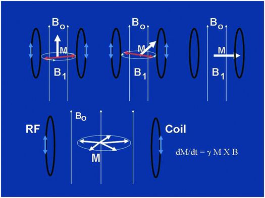
Figure 29.2 The top row shows a depiction of the tipping of the magnetization vector M of the sample from its equilibrium position oriented along the main magnetic field H_o (thousands of Gauss), to its nonequilibrium position in the transverse plane perpendicular to H_o, all accomplished by the little oscillating magnetic field H₁ (<1 Gauss) precessing in the transverse plane and applied at just the right (Larmor) frequency with a transmit coil. The bottom cartoon depicts the precession of M at the Larmor frequency following the tipping, or “excitation” into the transverse plane. This causes a magnetic flux through the receiver coil and, hence, via Faraday’s law of induction, a time-varying voltage in the receiver coil, which is the signal we detect with RF apparatus. Modern MR scanners operating at high-field strengths, 1.5 T or 3 T, bracket the radio FM band, operating at or near 64 MHz and 128 MHz, respectively.

Once in the transverse plane following an RF pulse, the spins precess for a period of time during which they also re-orient themselves (“recover”) back into alignment with the main magnetic field. During this time they also lose coherence with each other as they do not all precess at exactly the same frequency, but this is discussed in more detail below. From the signal perspective, as long as coherent precession is occurring, any coil that is oriented perpendicular to the main field, as shown in the lower row of Fig. 29.2, will experience an oscillating magnetic field flux resulting from the precession of the spins. This changing magnetic flux in turn results, through Faraday’s law of induction named after Michael Faraday (1791–1867), in an oscillating electrical current within the coil that is amplified and detected as a time varying voltage – the “signal” from the sample. Such signals are measured (following demodulation with a “carrier frequency” as in FM radio) and stored in dedicated computers, another essential hardware component of MRI scanners, for subsequent image reconstructions. Note that both the tipping and the precessing of spins, associated with the RF transmission and reception acts of MR respectively, occur only at or close to the Larmor frequency, or “on resonance,” justifying the R in NMR and MRI.

Tipping, or “exciting,” the spins and listening to the resulting signal via their precession in the transverse plane brings us up to about 1980, at which point the NMR experiments begun in the 1940s began to become the MRI experiments heralding the modern era. This miracle required the addition of some specific hardware to allow for the spatial localization of the spins, or what we call “imaging.” That is, in the good old days before 1980 or so, a signal was generated from the entire object in the bore of NMR magnets, primarily located in chemistry and physics departments of colleges and universities. This signal carried useful information such as the chemical contents or properties related to the microstructure of the interrogated object. However, these signals did not emanate from specific parts of the object (at least not intentionally) nor did they carry specific information regarding where the spins were and were not within the bore of the scanner. The addition of magnetic field gradients applied across the sample changed all that, garnering the 2003 Nobel prize for Paul Lauterbur (1929–2007) and Sir Peter Mansfield, two of the pioneers in the use of gradient technology for MRI. Magnetic field gradients are designed to allow for selective excitation of “slices” or “slabs” of spins and to further encode the resulting signals with spatial information as to the location of the spins within the excited volumes. These gradients are measured in Gauss/centimeters and of which a minimum of three are needed for x-, y-, and z-axis spatial localization of signals, e.g., imaging, causing spatially dependent, highly controlled, deviations in B_o. These deviations in turn cause spatially dependent changes, on the order of kHz, to the Larmor frequency and make the signals received and/or the spins tipped depend on their location in space. The gradient coils used for MRI are engineering marvels that have, over the last three decades, evolved into fairly standardized units. They probably will not evolve any further due to physiologic constraints. For example, how quickly gradients can turn on and off (“slew rates” or “rise times” in the vernacular) and how strong they are (maximum gradient amplitude in Gauss/cm) play important roles in how quickly images can be made and also how detailed the images can be as governed by the “spatial resolution.” Modern values for these crucial gradient parameters are, however, close to the thresholds at which peripheral nerve stimulation can be evoked (10), which largely limits further engineering refinements for achieving more powerful gradient coils, at least for human imaging. The coils now, however, provide excellent linearity of magnetic field gradients over all three axes and permit generation of submillimeter spatial resolutions in clinically reasonable scan times. (Rule of thumb: no one wants to be in the bore of a magnet for more than an hour.)

How do we use gradients and signals to make images? Though there are a range of possibilities, the most common method is to perform two-dimensional Fourier transform (2D-FT) imaging, though three-dimensional Fourier transform (3D-FT) imaging formats are also used for several applications. In 2D-FT formats, a “slice selection” gradient, conventionally referred to as the “z-gradient” though its axis in space is completely selectable using combinations of the “laboratory frame” x-, y-, and z-gradients, is applied during the RF pulse. This effectively limits the spins, which are tipped into the transverse plane to a “slice” of the object. The nominal thickness of the slice, generally between 2 and 10 mm depending on the clinical application, is a function of both the strength of the slice selection gradient as well as the specific shape or “envelope” of the RF pulse applied (11). Following “slice selection,” signals are recorded, which are both “phase encoded” and “frequency encoded,” to begin to gather the information necessary to form a 2D image of the selected slice (6). Phase encoding refers to the process of applying, for a brief period of time τ_p, a gradient of fixed amplitude along the “y-axis” perpendicular to the slice select “z-axis.” Following this “phase-encode blip,” a signal is “read out” while a frequency encoding gradient is applied along the x-axis perpendicular to the y- and z-axes.

To gather enough information to generate a 2D-FT image, this entire process – slice selection, phase encoding, and frequency encoding – must be repeated m times where m is one of two numbers of the in-plane image matrix of n × m values, for example 256 × 256. The only difference between successive signal collections is the amplitude of the phase encode gradient which takes on a total of m values, both negative and positive around a very low, or no (zero), phase encode amplitude value. The n in the image matrix refers to the number of frequency samples, that is how many times during each signal collection the transverse magnetization gets measured. For example, an 8 millisecond (ms) signal readout may utilize an n of 256 digital samples, requiring a new digital sample every 31 microseconds (μs), a rather small unit of time referred to as the “dwell time” in the older literature and inversely proportional to the full receiver bandwidth (BW) of ±16 kHz in this case. In 2D-FT imaging, a single slice is sampled for a signal and then, immediately afterwards, a different, adjacent or nearby, slice is sampled and so on. One returns to the first slice sampled to get another signal from that slice after a time known as the repetition time (TR), a time which, as I discuss further below, also plays an important role in tissue contrast as it determines how long we let each slice “relax” after disturbing it from equilibrium. Thus, in conventional 2D-FT imaging, multiple slices are sampled each TR period and the total scan time for a multislice acquisition is m (the number of phase encodes) × TR, when only a single “signal average” is used. In 3D-FT imaging, a much thicker slice, or “slab” of spins is tipped down into the transverse plane and two phase encoding procedures are applied, one for the z-axis and one for the y-axis so that the total scan time is m × l × TR where l is the number of slices encoded along the z-direction. In general 3D-FT imaging provides a higher signal-to-noise ratio (SNR) than 2D-FT imaging at the expense of scan time due to the nested phase-encode looping required (e.g., for every single slice encode we have to do m phase encodes).

How do the signals that we collect, which are nothing but time varying voltage changes, get decoded into images once collection is complete? This is where the Fourier transform, the FT in 2D-FT and 3D-FT imaging and named after the French scientist/soldier Jean Baptiste Joseph Fourier (1768–1830), comes into play. A Fourier transform is a mathematical operation that extracts the frequency content of signals that vary with some parameter. For the frequency-encode direction this parameter is time throughout signal readout, while for the phase-encode direction this parameter is effectively the phase-encode gradient amplitude (5). Basically the frequency contents of the signals as functions of time and the phase-encode gradient amplitude reveal the locations of spins within the selected slice in 2D-FT imaging or within the entire 3D volume in 3D-FT imaging. Thus, what is stored in the computer as a series of signals, the “k-space” domain as it is often referred to, is transformed or reconstructed into an image via the magic of the FT – thank you Jean Baptiste! Some k-space data and their FTs are shown in Fig. 29.3 and demonstrate what happens when sections of k-space are not sampled. On the left of Fig. 29.3, one sees a full sampling of k-space whose FT in the top row is a decent axial image of a brain. Collecting only the central lines of k-space (middle), corresponding to the low phase-encode steps, results in a blurry image with contrast details like the differentiation between cerebrospinal spinal fluid (CSF) and brain parenchyma intact. Leaving out the central lines in k-space and collecting the outer lines in k-space (high-positive and negative-phase encodes) results in an image with few contrast details but sharp edges, as the outer lines of k-space contain information regarding the high-frequency components of an image (right column).

Figure 29.3 Axial images of a brain (top row) and the signals from which they were reconstructed (bottom row) referred to as the k-space representations or just “k-space.” Each horizontal line in k-space is a signal acquired as a GE or SE in conventional 2D-FT imaging, and the only difference between the lines is the strength of the phase-encode gradient, which preceded collection of the echo signal. The second and third columns show the effects of not collecting either the top and bottom k-space lines or the central k-space lines, respectively.

Figures 29.2 and 29.3 capture the essentials of imaging with MR; signals are generated with RF components (coils, amplifiers, etc.) and manipulated with magnetic field gradient coils to generate k-space data sets that can be further manipulated, via the FT operation, to visualize an image. Over the last decade or so a synthesis of RF receiver coil arrays have been combined with the gradient coil manipulations so that partial k-space data sets can in fact be acquired and reconstructed with much more fidelity than the examples shown in Fig. 29.3. This approach, in which multiple receiver coils are placed around the object and the individual coil sensitivities are used for spatial localization in addition to the gradient manipulations, is known as “parallel imaging” and has become quite common with scan times routinely being reduced by factors of two or more (12). A full description is beyond the scope of this work but, in some sense, the physiologic constraints of gradient switching (10) have led to innovative and creative use of multiple RF receiver coil technology to further advance the cause of fast imaging.

One final but important word on the “Us” part of image generation has to do with the types and the timings of the signals we collect following excitation. The two types of signal we most always collect are either “gradient echoes” (GEs) or “spin echoes” (SEs). The timings of the echo signals, the echo time or TE, refers to how soon after the initial tipping comes the center, or “refocusing” of the echo. Though both types of echoes are gainfully employed, there is a fundamental difference in how they are generated and how they are affected by forces beyond our control. In particular, one finds that when metallic implants, tissue/air or bone/tissue interfaces are present, GEs suffer from signal losses which are to a large degree compensated for in SEs. Figures 29.4 and 29.5 have been designed to show not only how each type of echo is generated but also why additional gradients caused by “susceptibility mismatches” from metallic implants, etc., influence GEs but not, to first order, SEs.

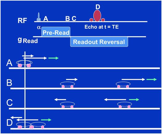
Figure 29.4 The fundamental manipulations we perform when acquiring gradient are shown in the top two lines. A RF slice-selective pulse (slice-selective gradients not shown) is played out followed by a frequency encode gradient, which consists of a pre-read section whose polarity is reversed for the “readout,” e.g., when we collect the signal for, say 256 “dwell times.” Points A, B, C, and D within this sequence are depicted as a car race between two cars in the lower four lines. The white arrows depict the velocities of each car due to the frequency-encode gradient, assuming the cars are at different locations along this gradient. When reversed the fast car begins to catch up with the slow car (point C) but the little blue arrow at the location of one car does not reverse, which may be due to a metallic implant or air/tissue interface that we don’t control. As a consequence, the refocusing we are trying to perform with the frequency-encode reversal alone is not sufficient to cause a perfect refocusing of the two cars at point D.

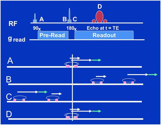
Figure 29.5 Same as in Fig. 29.4 but for a spin-echo sequence of events. Note how the refocusing pulse applied between time points B and C magically moves the two cars to mirrored positions along the starting line so that the fast car now is behind the slow car and, even with the additional gradient from the little blue arrow, catches up perfectly with the slower car at time point D. There is no frequency-encode gradient reversal in this case, it is rather as if the 180-degree refocusing pulse reversed all the gradients in the system, those we do and those we do not control. This is the fundamental difference between GEs and SEs.

The top two lines of Fig. 29.4 show the essentials of the pulse sequence that will result in a GE. A slice-selective RF pulse of flip angle α (slice-select gradient not shown) tips some of the magnetization into the transverse plane whereupon the frequency-encoding gradient is applied with a positive polarity (time point A). The spins then precess at different speeds according to their location along the frequency encoding axis for a specified period of time – up to time point B. This is depicted by a two-car race analogy in Fig. 29.4 in which, at time point A, one car is associated with a big white arrow and the other a little white arrow denoting their different speeds due to their different positions along the frequency-encode gradient axis. Note we have added a little blue arrow to one of the cars. We will attribute this to a metallic implant near this car, but not the other, which will add to the speed of this car in a manner beyond our control. The time between A and B is referred to as the pre-readout time as it is designed to allow the spins to dephase (cars to separate) for a period prior to our collecting, or reading out, the signal. At time point C the frequency-encode gradient is reversed to a negative polarity causing the spins to precess in the opposite direction, but also with speeds depending on where they are along the frequency-encoding axis. In the car race analogy, the reversal of the frequency gradient is represented by the reversal of the white arrows at time point C. The little blue arrow, being a gradient we do not control, does not reverse and now works against the big white arrow in this phase of the race. In its absence (only white arrows) the fast car would catch up perfectly to the slow car at time point D, defined as the center of the GE or the TE time after the α pulse. Because of the little blue arrow not reversing direction, however, one car went faster than it should between A and B, and then slower than it should have between C and D, resulting in an incomplete “refocusing” at echo time D.

In the case of a SE, a rather magical reversal of all the gradients in the system, those within and without of our control, is accomplished with the use of a refocusing or “180 degree” RF pulse applied at time point C, as shown in Fig. 29.5. The polarity of the frequency-encode gradient never switches in the SE sequence but rather the 180-degree pulse moves the fast and slow cars to mirror positions along the starting point at time point C. They then proceed to race at their same respective speeds before and after the pulse. Thus, whether or not an additional gradient (little blue arrow again) is present, a perfect refocusing at time point D occurs, as depicted in Fig. 29.5.

The car race analogies just provided for GE and SE formation are of course somewhat simplified as one knows that in any real race there will be random variations in speeds during the first versus the second half of any race. In the case of individual spins, such random variations in precession frequencies are caused by encounters with time varying microscopic fields from neighboring spins on water molecules, proteins, membranes, etc., and lead to incomplete refocusing in both GEs and SEs. The fundamental differences and similarities between GEs and SEs are discussed further below in the context of the two transverse relaxation times, T2* and T2, and the difference between “reversible” and “irreversible” transverse relaxation processes affecting “Them” (13). What each type of echo shares, however, is a pre-selected “echo time” or TE which, like TR, plays a major role in the soft tissue contrast observed. The TEs may be made short, on the order of a few ms, or long and on the order of 70–120 ms with the long and short defined here in reference to the tissue transverse relaxation times T2* or T2. In practical terms, T2* loosely refers to how quickly signals from a distinct “voxel” disappear with TE in GE acquisitions while T2 refers to how quickly these signals disappear with TE in SE acquisitions. But these transverse relaxation times, as well as the characteristic time with which the spins in a voxel return to equilibrium along the main field B_o, the T1 or longitudinal relaxation time, are more properly discussed in the context of “Them,” not “Us,” as I now proceed to do.

“Them”

Having established that water is very prevalent in the human body, constituting the primary constituent of most tissues and organs, we now must ask what are these water molecules experiencing within the many different environments in tissue, both normal and pathologic? In turn, how do these different environments influence water signals as we image them, resulting in the rich tissue contrast observed?

A simple example helps set some extremes of the environments available to water and demonstrates how much signal can be affected by different environments. Consider the image of the cup of water with an ice cube floating in Fig. 29.1. One can plainly see the fluid water as bright while the ice cube is a dark void, despite the fact that both the fluid water and the ice have very similar densities of hydrogen atoms. By freezing the water, the internal motion of the water molecules, both rotational and translational, is dramatically reduced compared to water molecules within the liquid phase. The freezing means that the tiny magnetic fields generated by the protons themselves are not time averaged to zero on the time scale of the MR experiment like they are in the liquid state, where water molecules are tumbling and translating on time scales of the order of every 10^–12 seconds (a picosecond). As a consequence, in the solid there is a large range of static, local microscopic fields among the individual protons. This in turn creates a large static frequency distribution centered on the primary Larmor frequency associated with the main field B_o. This frequency distribution means that the signal from the entire spin ensemble within any voxel sized region “dephases” very quickly, e.g., the signal disappears very quickly. In the liquid on the other hand, the rapid tumbling and bodily translation of the protons results in random, dynamic local magnetic fields which average towards zero well within the timescale of our signal-generating capabilities, leaving the local field B_o as the major player. As such, the ensemble of spins within any given liquid voxel remains “in phase” much longer than in ice, resulting in a signal that precesses coherently for a relatively much longer time at the Larmor frequency.

The example of water versus ice dramatically demonstrates how the tumbling or rotating of water molecules and their bodily translational motions through space, or diffusion, affect their signal strength in an image. Indeed, anything that causes restrictions of these microscopic motions alters the water signal. Within tissue there are many such possible sources of water restriction such as cell membranes, macromolecules, proteins, etc., all of which can hinder the microscopic motions of water and provide sources of local microscopic magnetic field fluctuations at relevant frequencies. The microscopic details of a water molecule’s interactions with such tissue constituents play a large role in determining the degree of motional restriction. A water molecule may transiently become part of a hydration layer of a macromolecule or membrane, taking on the rotational and translational properties of the latter moiety. It may also participate in a single hydrogen bonding arrangement with an amine or hydroxyl group, leaving it free to rotate about one axis while considerably restricting its motional freedom compared to a water molecule in the pure solvent or “bulk” water phase. Clearly the devil is in the details when one ponders the amalgam of interactions available to a water molecule in tissue, each of which has specific effects on the rotational and translational motions that affect the signal intensity we observe in any given image. To add to the complexity it must be noted that there may be, and often is, paramagnetic species causing large amplitude local fluctuating magnetic fields, particularly de-oxygenated hemoglobin of blood or the gadolinium contrast agents we (Us again!) inject, which alter the local magnetic environment which water molecules see and, in turn, the water signal.

The more general manner in which we have come to understand the water signal as a function of its local environment and the manner in which we have learned to manipulate this signal to our advantage in diagnosing various conditions is through the concept of the so-called “relaxation times.” There are three basic relaxation times to consider. The first is the longitudinal relaxation time T1, also referred to as the spin-lattice relaxation time, which is associated with the return of the magnetization to its equilibrium position along B_o after it has been tipped away from this position. The second is the transverse relaxation time T2*, which is associated with the dephasing of the individual spins in the transverse plane after a good tipping with an RF pulse and left undisturbed by additional pulses. The third is the transverse relaxation time T2, which represents the eventual dephasing of spins despite efforts to rephase them with an additional refocusing pulse as in the SE sequence of Fig. 29.5. I discuss each of these three relaxation times in turn and then focus, in the “Us and Them” section, on how we design pulse sequences to emphasize each of them for different tissue contrast options.

When considering T1 relaxation, one must recall that to get spins tipped down into the transverse plane from their equilibrium position along B_o we used an RF pulse of just the right frequency, the resonance or Larmor frequency. This is in fact exactly how they must also be returned to equilibrium but without our help. That is, they must experience local microscopic magnetic field fluctuations at or near the Larmor frequency in order for them to flip back up along the main field axis. These magnetic field fluctuations, around 65 MHz for 1.5 T and 130 MHz for 3.0 T imaging systems, will of course be caused by whatever the local environment is that is seen by our water molecules. For example, in liquid water at room temperature where the local field fluctuations due to tumbling and bodily spin translational motions (e.g., diffusion, vide infra) are generally much higher than typical Larmor frequencies, the return to equilibrium is relatively slow and on the order of several seconds, a long T₁. Similarly in ice the return to equilibrium is also slow and also on the order of several seconds but for entirely different reasons, as first noted over 60 years ago by Bloembergen, Purcell, and Pound (1948). Edward Purcell (1912–1997) shared the 1952 Nobel Prize with Felix Bloch, while Nicolaas Bloembergen (1920–) shared the 1981 Nobel prize, and one read of the classic 1948 paper on relaxation (14) may help explain why. Back to ice though, in which the tumbling and diffusional motions have been largely frozen out or at least slowed way down. This leaves very few magnetic field fluctuations at or near the much higher Larmor frequencies need in the MHz range to provide efficient mechanisms for the return to equilibrium, e.g., a long T1 again just like in liquid water but for different reasons.

Of course tissue is neither ice nor water but, from a water molecule’s perspective, something in between, not frozen as in ice but certainly hindered in its rotational and translational motions compared to pure water (15). This leads to typical tissue longitudinal relaxation times shorter than those in our two extreme examples, generally in the 500–2000 ms range. Lipid T1 values are even smaller, in the 200–400 ms range, as the large sizes of the hydrocarbon chains mean their tumbling and diffusional rates are closer to the imaging Larmor frequencies, causing efficient mechanisms for the return to equilibrium. In tumors, it is often found that more “free water” results in longer T1 and also T2 values than the host tissues, allowing for excellent tumor detection. The effect is obviously critical to MRI’s enormous success in oncologic applications and was arguably first reported in context by Raymond Damadian in the early 1970s (16) who energetically sought to make, and made, the first human MR image as documented in an interesting book by Kleinfield (17).

As with T1, the transverse relaxation times T2*and T2 also play significant roles in tissue contrast in SE-based and GE-based imaging, respectively. Factors affecting T2* include any static frequency distributions present within the voxel, such as those we encountered with the wide range of local magnetic fields in ice. Such static frequency distributions are also found in voxels near metallic implants, braces, clips, air/tissue and/or tissue/bone interfaces. In addition, T2* is affected by the time varying magnetic field fluctuations associated with random encounters each water molecule proton has with the local magnetic fields generated by other water molecules, proteins, membranes, etc. Broadly speaking, these factors may be separated into what are thought of as “reversible” relaxation processes, from static frequency distributions, versus “irreversible” relaxation processes from randomly varying local magnetic fields (13). The distinction is critical for understanding the transverse relaxation time T2, and how it differs from T2*. The time constant T2 refers to how quickly the transverse magnetization decays despite efforts to retain and/or resuscitate it by using additional RF “refocusing” pulses to gather “spin echoes” following the initial tipping of the magnetization into the transverse plane. Essentially, a refocusing pulse serves to reverse the dephasing of spins caused by static frequency distributions present within a voxel. Refocusing pulses cannot, however, restore dephasing due to random fluctuations of the local magnetic fields encountered by the spins during the course of the measurement, as these will be different before and after each refocusing pulse. Thus, the primary difference between T2* and T2 is that the former is affected by both “reversible” relaxation mechanisms caused by intrinsic frequency distributions, such as encountered when voxels are placed near metallic hardware, braces, clips, air/tissue interfaces, etc., as well as “irreversible” relaxation processes while the latter is primarily affected only by the irreversible relaxation processes. This distinction between T2*and T2 is most famously taken advantage of by “Us” when we decide to generate either “gradient echo” images or “spin echo” images, as discussed above in Figs. 29.4 and 29.5 with the car race analogy. Figure 29.6 illustrates gradient- versus spin-echo-based acquisitions of an axial brain slice in which susceptibility dephasing was deliberately introduced with a paper clip appended to the forehead (don’t try this at home!) along with a coronal abdominal GE image through the posterior section of a subject wearing sweat pants with the vender logo (“Hollister” I believe), which contains some ferrous dye material. The brain image with the substantial loss of signal anteriorly due to the paper clip was acquired using a series of GEs in an echo planar imaging (EPI) diffusion scan (18). This signal was substantially restored using a line scan diffusion imaging (LSDI) approach (19, 20), which, though much slower, relies on the acquisition of a SE for each vertical line in the image. The loss of signal accompanying the ferrous dye logo in the coronal abdominal GE image is typical of signal loss in GE imaging caused by susceptibility-based mismatches which introduce gradients at locations which we do not control and which, in this case, may have unintended advertising consequences.

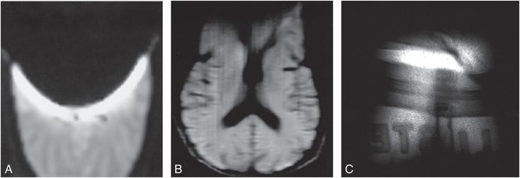
Figure 29.6 A, B, The two axial brain images were acquired with a paper clip appended to the forehead of the subject, the left image (A) with an echo-planar readout consisting of multiple GEs and the middle image (B) with a line scan imaging approach that utilized a single SE for each vertical column. Note the major loss of signal towards the anterior of the brain in the GE image-based acquisition compared to the SE-based acquisition, a consequence of a failure to rephase reversible dephasing mechanisms in GE acquisitions, such as that caused by susceptibility mismatch and subsequent uncontrolled gradients associated with the paper clip. C, The far right image is a GE acquisition in which the ferrous dye containing logo of the subject’s pants cause signal loss in the tissue, allowing one to partially diagnose the pant’s vendor as “Hollister.”

I have emphasized how the relaxation times are influenced by the rotational and translational motions of the water molecules and, in addition for T2*, static frequency distributions. One additional parameter related to the translational motions alone is worthy of discussion in the context of “Them,” and this is the so-called apparent diffusion coefficient, or ADC, and some related considerations of water diffusion in tissue. If one were able to label a water molecule’s location at some time point and then, say 80 ms or so later, inquire as to its new position then one would have a measure of how far the water molecule “diffused” in that time. This is, broadly speaking, what so-called diffusion-weighted imaging (DWI), and its cousin diffusion tensor imaging (DTI), does. Namely, we can sensitize the signals we collect for MR images to the tissue diffusion coefficients of the water molecules (19–22) within a voxel and generate images based on the diffusive properties of water. In tissue the motion of water can be very complicated and can be isotropic, that is free to diffuse in any direction rapidly and equally as in a large cyst or a cup of coffee (23), for example. On the other hand, the microscopic motion may be “anisotropic,” which is more likely to diffuse along one direction than others as in white matter fiber tracts (24). In addition, even if the motion is isotropic, it can be restricted or confined by cell membranes, at least to some degree depending on the water permeability of the cell membrane. Water diffusion in tissue is an extremely complicated topic which includes not only restricted, anisotropic diffusion but also the perfusive motions of blood within capillary beds (25). Despite the complexity, the advent and use of diffusion imaging now plays a significant clinical role particularly in identifying hypoxic ischemic injury and other less well-understood parenchymal insults occurring with abusive head trauma (AHT). Signals are sensitized to water diffusion with the same magnetic field gradients used to encode spatial information so in many ways MRI scanners are particularly well adapted for making diffusion measurements along different directions and I shall discuss this further in the “Us and Them” section. For now it is important to note that the translational motion of water molecules, their “diffusion,” not only influences relaxation times but can be probed directly for diagnostic information with diffusion imaging approaches and so represents tissue contrast parameter(s) separate from, if related to, the primary relaxation times.

Some biology please!!!

One of an author’s duties is to occasionally recall the title of the piece being written and to try to adhere to it. In this regard the astute reader may note how the above descriptions of hardware, signals, relaxation times, etc., have largely emphasized the physics over the biology of MRI so perhaps the time has come to attempt a rebalance. Different organs and the tissues of which they are composed have different biologic purposes in sustaining life, or courting sickness and death. The cells of different organs and invasive pathologies differ in function and, in turn, in size, shape, and internal organelles and macromolecular composition. Similarly the relative density of cells, or equivalently the volume percentage of intracellular versus extracellular space, will vary from tissue to tissue as will the vascularity and overall blood volume. These “compartments,” intracellular, extracellular, and the vasculature, all present different environments for water molecules each with arguably different relaxation properties. In addition, during the course of measurement, water molecules may “exchange” between these various compartments. Thus one can expect that the relative proportions of the three compartments within an imaged voxel will play an important role in the MR signal intensity – as will the relative water/membrane permeabilities and subsequent water exchange rates between compartments. From a basic science perspective, it has long been, and remains, a goal to determine how much detailed information regarding relative compartment sizes and water exchange rates between compartments can be gleaned from quantitative MR studies of tissue. From a clinical perspective, however, it is enough to appreciate that such properties play a big role in MRI and that inferences regarding these properties often aid in diagnostic interpretation. In this context, some exemplary important organs/tissues, blood, brain, and bone marrow, and the specific biologic properties that cause them to have very different MRI appearances, apart from their shape(s) and position in the body, are discussed.

Brain

The human brain, arguably the most advanced example of the evolutionary process on this planet, presents a somewhat complex environment for water molecules but with some fairly basic tissue “segmentation” rules. Apart from the large blood vessels accessible with MR angiography (MRA) techniques (Fig. 29.7), the three basic “segmentable” tissue types in the brain which are of most relevance for MR interpretations are the CSF and the two brain parenchymal components gray and white matter. Normal CSF is practically pure water in which the water molecules are free to tumble and diffuse rapidly and so, as in pure water, have very long relaxation times (>2 s). Protein and/or blood introduced into the CSF from pathologic processes will shorten these relaxation times. In gray and white matter, most of the water (~80%) is intracellular, thus spending less time in the smaller extracellular space including the vasculature, which is higher in gray than in white matter. In mature white matter, the myelinated axons provide a restricted environment for some water molecules and, to varying degrees, restrict the diffusional motion of water molecules as may be assessed with DWI and DTI techniques (vide infra). The restrictions also reduce the relaxation times of white matter compared to gray matter and allow for excellent differentiation between the two on T1- and/or T2-weighted SE images, as shown in Fig. 29.8. Newborn brains and/or fetal brains (Fig. 29.9) are very different from adult brains and the maturation process from very watery beginnings with longer relaxation times to drier, more myelinated tissues with age has been well documented (26–28) and shows up profoundly in MR images. A correlation of the development of the brain structures with age (0–18 years) as determined from MRI with psychologic development was the focus of a fairly recent, major National Institutes of Health (NIH) multicenter study (29). The conspicuity of tumors, ischemic strokes, vasogenic hemorrhage, edema, etc., on MR images all reflect the altered environment that water molecules are experiencing within these pathologies, each with its own story and each too long to tell here.

Figure 29.7 An MR angiogram presented as a MIP display showing the major blood vessels of the brain. This image is from a time-of-flight (TOF) approach using a four-slab 3D-spoiled GE acquisition in which spins from static tissue are suppressed by T1 saturation while in-flowing “unsaturated” blood spins yield a large signal.

Related posts:

Abusive head trauma: intracranial imaging strategies Differential diagnosis V: obstetric trauma The skeleton: structure, growth and development, and basis of skeletal injury Differential diagnosis VI: normal variants Bony thoracic trauma Upper extremity trauma

Stay updated, free articles. Join our Telegram channel

Join