Treatment Planning I: Isodose Distributions

The central axis depth dose distribution by itself is not sufficient to characterize a radiation beam that produces a dose distribution in a three-dimensional volume. In order to represent volumetric or planar variations in absorbed dose, distributions are depicted by means of isodose curves, which are lines passing through points of equal dose. The curves are usually drawn at regular intervals of absorbed dose and may be expressed as a percentage of the dose at a reference point. Thus, the isodose curves represent levels of absorbed dose in the same manner that isotherms are used for heat and isobars, for pressure.

11.1. ISODOSE CHART

An isodose chart for a given beam consists of a family of isodose curves usually drawn at equal increments of percent depth dose, representing the variation in dose as a function of depth and transverse distance from the central axis. The depth dose values of the curves are normalized either at the reference point of maximum dose on the central axis or at a fixed distance along the central axis in the irradiated medium. The charts in the first category are applicable when the patient is treated at a constant source to surface distance (SSD) irrespective of beam direction. In the second category, the isodose curves are normalized at a certain depth beyond the depth of maximum dose, corresponding to the axis of rotation of an isocentric therapy unit. This type of representation has been used in the past for treatment planning of rotation therapy and isocentric treatments, before the advent of computer treatment planning. Figure 11.1 shows both types of isodose charts for a ⁶⁰Co γ-ray beam.

Examination of isodose charts reveals some general properties of x-ray and γ-ray beam dose distributions.

The dose at any depth is greatest on the central axis of the beam and gradually decreases toward the edges of the beam with the exception of some linac x-ray beams, which exhibit areas of high dose or “horns” near the surface in the periphery of the field. These horns are created by the flattening filter, which is usually designed to overcompensate near the surface in order to obtain flat isodose curves at greater depths.
Near the edges of the beam (the penumbra region), the dose rate decreases rapidly as a function of lateral distance from the beam axis. As discussed in Chapter 4, the width of geometric penumbra, which exists both inside and outside the geometric boundaries of the beam, depends on source size, distance from the source and source to diaphragm distance.
Near the beam edge, falloff of the beam is caused not only by the geometric penumbra, but also by the reduced side scatter. Therefore, the geometric penumbra is not the best measure of beam sharpness near the edges. Instead, the term physical penumbra may be used. The physical penumbra width is defined as the lateral distance between two specified isodose curves at a specified depth (e.g., lateral distance between 90% and 20% isodose lines at the depth of D^max).
Outside the geometric limits of the beam and the penumbra, the dose variation is the result of side scatter from the field and both leakage and scatter from the collimator system. Beyond this collimator zone, the dose distribution is governed by the lateral scatter from the medium and leakage from the head of the machine (often called therapeutic housing or source housing).

Figure 11.2 shows the dose variation across the center of the field at a specified depth. Such a representation of the beam is known as the beam profile. It may be noted that the field size is
defined as the lateral distance between the 50% isodose lines at a reference depth. To ensure that this agrees with the field size defined by the field-defining light, a procedure called beam alignment is performed in which the field-defining light is made to coincide with the 50% isodose lines of the radiation beam projected on a plane perpendicular to the beam axis and at the standard SSD or source to axis distance (SAD).

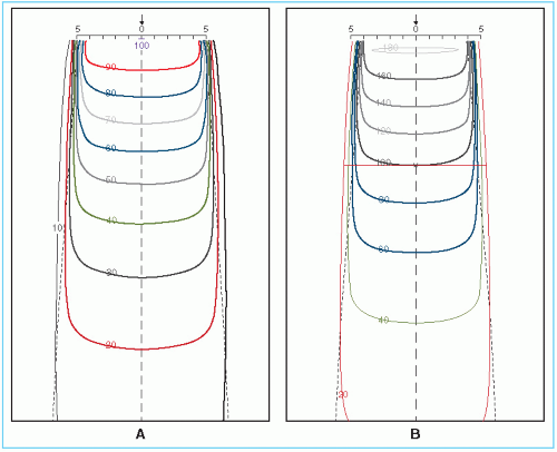Figure 11.1. Example of an isodose chart. A: Source to surface distance (SSD) type, ⁶⁰Co beam, SSD = 80 cm, field size = 10 × 10 cm² at surface. B: Source to axis distance (SAD) type, ⁶⁰Co beam, SAD = 100 cm, depth of isocenter = 10 × 10 cm². (Data from University of Minnesota Hospitals, Eldorado 8 Cobalt Unit, source size = 2 cm.)

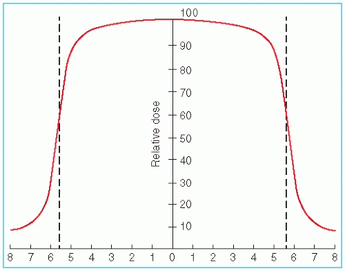Figure 11.2. Dose profile at depth showing variation of dose across the field. ⁶⁰Co beam, source to surface distance = 80 cm, depth = 10 cm, field size at surface = 10 × 10 cm². Dotted line indicates geometric field boundary at a 10-cm depth.

Another way of depicting the dose variation across the field is to plot isodose curves in a plane perpendicular to the central axis of the beam (Fig. 11.3). Such a representation is useful for treatment planning in which the field sizes are planned on the basis of an isodose curve (e.g., 90% to 95%) that adequately covers the target volume.

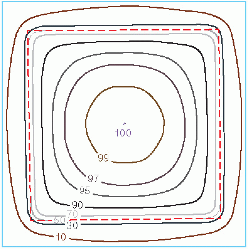Figure 11.3. Cross-sectional isodose distribution in a plane perpendicular to the central axis of the beam. Isodose values are normalized to 100% at the center of the field. The dashed line shows the boundary of the geometric field.

11.2. MEASUREMENT OF ISODOSE CURVES

Isodose charts can be measured by means of ion chambers, solid state detectors, or radiographic films (Chapter 8). Of these, the ion chamber is the most reliable method, mainly because of its relatively flat energy response and precision. Although any of the phantoms described in Chapter 9 may be used for isodose measurements, water is the medium of choice for ionometric measurements. The chamber may be waterproof or covered by a thin plastic sleeve that covers the chamber as well as the portion of the cable immersed in the water.

Ionization chamber used for isodose measurements should be small so that measurements can be made in regions of high dose gradient, such as near the edges of the beam. It is recommended that the sensitive volume of the chamber be less than 15 mm long and have an inside diameter of 5 mm or less. Energy independence of the chamber is another important requirement. Because the x-ray beam spectrum changes with position in the phantom owing to scatter, the energy response of the chamber should be as flat as possible. This can be checked by obtaining the exposure calibration of the chamber for orthovoltage (1 to 4 mm Cu) and ⁶⁰Co beams. A variation of less than 5% in response throughout this energy range is acceptable.

Automatic devices or beam scanning systems exist for rapid measurement of the isodose curves. These systems are computer driven and measure dose distribution in a water phantom using computer software. Basically, the apparatus (Fig. 11.4) consists of two ionization chambers,
referred to as the detector A (or probe) and the monitor B. Whereas the probe is arranged to move in the tank of water to sample the dose rate at various points, the monitor is positioned in the beam at some fixed point in the field to monitor the beam intensity as a function of time. The ratio of the detector to the monitor response (A/B) is recorded as the probe is moved in the phantom. Thus, the final response A/B is independent of fluctuations in beam output.

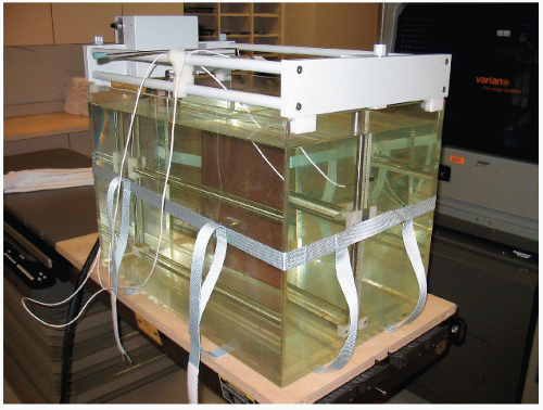Figure 11.4. Photograph of a water phantom.

In the water phantom, the movement of the probe is controlled by the beam-scanning computer. The probe-to-monitor response ratio is sampled as the probe moves across the field at preset increments. These beam profiles are measured at a number of depths, and the data thus acquired are stored in the computer in the form of a matrix that can then be transformed into isodose curves or other dose distribution formats allowed by the computer program.

For additional information regarding the design, setup and quality assurance of beam scanning systems, the reader is referred to the report of AAPM Task Group 106 (1).

11.3. PARAMETERS OF ISODOSE CURVES

Among the parameters that affect the single-beam isodose distribution are beam quality, source size, beam collimation, field size, SSD, and the source to diaphragm distance (SDD). A discussion of these parameters will be presented in the context of treatment planning.

A. BEAM QUALITY

As discussed previously, the central axis depth dose distribution depends on the beam energy. As a result, the depth of a given isodose curve increases with beam quality. Beam energy also influences isodose curve shape near the field borders. Greater lateral scatter associated with very low-energy beams (e.g., orthovoltage) causes the isodose curves outside the field to bulge out. In other words, the absorbed dose in the medium outside the primary beam is greater for such low-energy beams than for those of higher-energy such as megavoltage beams.

Physical penumbra depends on beam quality as illustrated in Figure 11.5. As expected, the isodose curves outside the primary beam (e.g., 10% and 5%) are greatly distended in the case of orthovoltage radiation. Thus, one disadvantage of the orthovoltage beams is the increased scattered dose to tissue outside the treatment region. For megavoltage beams, on the other hand, the scatter outside the field is minimized as a result of predominantly forward scattering and becomes more a function of collimation than energy.

B. SOURCE SIZE, SOURCE TO SURFACE DISTANCE, AND SOURCE TO DIAPHRAGM DISTANCE—THE PENUMBRA EFFECT

Source size, SSD, and SDD affect the shape of isodose curves by virtue of the geometric penumbra, discussed in Chapter 4. In addition, the SSD affects the percent depth dose and therefore the depth of the isodose curves.

As discussed previously, the dose variation across the field border is a complex function of beam energy, geometric penumbra, lateral scatter, and collimation. In addition, as the beam energy increases in the megavoltage range, the lateral dose variation near the field borders is made more gradual because of increase in the range of laterally scattered electrons. Therefore, the field sharpness at depth is not simply determined by the source or focal spot size. For example, by using penumbra trimmers or secondary blocking, the isodose sharpness at depth for ⁶⁰Co beams with a source size of 1 to 2 cm in diameter can be made comparable with higher-energy linac beams, although the focal spot size of these beams is usually less than 2 mm. Comparison of isodose curves for ⁶⁰Co, 4 MV, and 10 MV in Figure 11.5 illustrates the point that the physical penumbra width for these beams is more or less similar.

C. COLLIMATION AND FLATTENING FILTER

The term collimation is used here to designate not only the collimator blocks or multileaf collimators that give shape and size to the beam, but also the flattening filter and other absorbers or scatterers in the beam between the target and the patient. Of these, the flattening filter, which is used for megavoltage x-ray beams, has the greatest influence in determining the shape of the isodose curves. Without this filter, the isodose curves will be conical in shape, showing markedly increased x-ray intensity along the central axis and a rapid reduction transversely. The function of the flattening filter is to make the beam intensity distribution relatively uniform across the field (i.e., “flat”). Therefore, the filter is thickest in the middle and tapers off toward the edges.

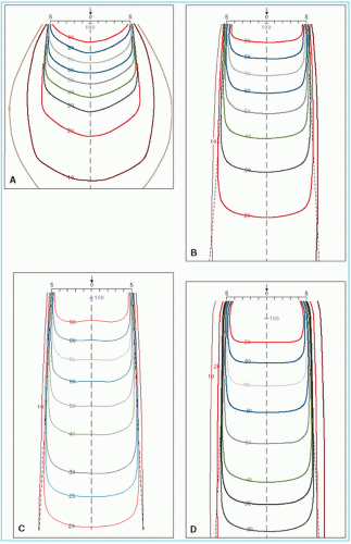Figure 11.5. Isodose distributions for different-quality radiations. A: 200 kVp, source to surface distance (SSD) = 50 cm, half-value layer = 1 mm Cu, field size = 10 × 10 cm². B:⁶⁰Co, SSD = 80 cm, field size = 10 × 10 cm². C: 4-MV x-rays, SSD = 100 cm, field size = 10 × 10 cm². D: 10-MV x-rays, SSD = 100 cm, field size = 10 × 10 cm².

The cross-sectional variation of the filter thickness also causes variation in the photon spectrum or beam quality across the field owing to selective hardening of the beam by the filter. In general, the average energy of the beam is somewhat lower for the peripheral areas compared with the central part of the beam. This change in quality across the beam causes the flatness to change with depth. However, the change in flatness with depth is caused by not only the
selective hardening of the beam across the field, but also the changes in the distribution of radiation scatter as the depth increases.

Beam flatness is usually specified at a 10-cm depth with the maximum limits set at the depth of maximum dose. This degree of flatness should extend over the central area bounded by at least 80% of the field dimensions at the specified depth or 1 cm from the edge of the field. By careful design of the filter and accurate placement in the beam, it is possible to achieve flatness to within ±3% of the central axis dose value at a 10-cm depth. The above specification is satisfactory for the precision required in radiation therapy.

To obtain acceptable flatness at 10 cm depth, an area of high dose near the surface may have to be accepted. Although the extent of the high-dose regions, or horns, varies with the design of the filter, lower-energy beams exhibit a larger variation than higher-energy beams. In practice, it is acceptable to have these “superflat” isodose curves near the surface provided no point in any plane parallel to the surface receives a dose greater than 107% of the central axis value (2).

D. FLATTENING-FILTER FREE (FFF) LINACS

In some cases, it may not be necessary to produce a flattened beam across a large (e.g., 40 × 40 cm²) field size. For example, linear accelerators designed only to deliver small fields, such as for radiosurgery treatments (c.f., Chapter 21), may not need a flattening filter to produce a beam that is sufficiently uniform. For treatments with intensity-modulated fields (c.f., Chapter 20), it is not necessary to flatten the beam prior to creating a variable intensity distribution. As a result, manufacturers are beginning to offer flattening-filter free (FFF) options on modern linear accelerators.

The largest difference between photon beams with and without flattening filters is seen in the cross-beam profiles. Beam profiles produced by FFF beams exhibit a central peak which is more pronounced with greater energy and field size. Because the photon energy spectrum in this case varies less with off-axis distance, profile shapes from FFF beams vary little with depth, typically by only a few percent (3). Percent depth doses are slightly lower than those from the flattened beams, due to the absence of beam hardening within the filter.

Beams produced without a flattening filter offer some advantages over conventional flattened beams. Without the presence of the attenuating filter, the incident photon fluence rate will increase by a factor to two or more, resulting in shorter treatment times. The removal of the filter will also reduce the scatter dose outside the field. The increased photon fluence per incident electron results in a lower neutron contamination per monitor unit, although for the lower photon energies used for radiosurgery and IMRT, this advantage is negligible.

For more information on the use of FFF linac beams, the reader is referred to the review of Georg et al. (4).

E. FIELD SIZE

Field size is one of the most important parameters in treatment planning. Adequate dosimetric coverage of the tumor requires a determination of appropriate field size. This determination must always be made dosimetrically rather than geometrically. In other words, a certain isodose curve (e.g., 90% to 95%) enclosing the treatment volume should be the guide in choosing a field size rather than the geometric dimensions of the field.

Great caution should also be exercised in using field sizes smaller than 6 cm in which a relatively large part of the field is in the penumbra region. Depending on the source size, collimation, and design of the flattening filter, the isodose curves for small field sizes, in general, tend to be bell shaped. Thus, treatment planning with isodose curves should be mandatory for small field sizes. In the case of ⁶⁰Co, the isodose curvature increases as the field size becomes overly large. The reason for this effect is the progressive reduction of scattered radiation with increasing distance from the central axis as well as the obliquity of the primary rays. The effect becomes particularly severe with elongated fields such as cranial spinal fields used in the treatment of medulloblastoma. In these cases, a complete isodose pattern is needed to assess dose uniformity or, at least, one should calculate doses at several off-axis points of interest.

11.4. WEDGE FILTERS

There are two classes of wedge filters: (a) physical wedge filters and (b) nonphysical wedge filters. A physical wedge filter is a wedge-shaped absorber that causes a progressive decrease in the intensity across the beam, resulting in a tilt of the isodose curves from their normal positions. As shown in Figure 11.6, the isodose curves are tilted toward the thin end, and the degree of tilt
depends on the slope of the wedge filter. In actual wedge filter design, the sloping surface is made either straight or sigmoid in shape; the latter design is used to produce straighter isodose curves.

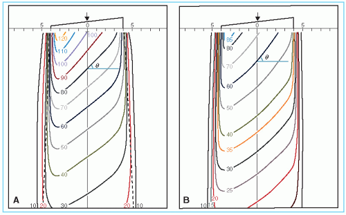Figure 11.6. Isodose curves for a wedge filter. A: Normalized to D^max. B: normalized to D^max without the wedge. ⁶⁰Co, wedge angle θ = 45 degrees, field size = 8 × 10 cm², source to surface distance = 80 cm.

A nonphysical wedge filter is an electronic filter that generates a tilted dose distribution profile similar to a physical wedge by moving one of the collimating jaws from one end of the field to the other. Nonphysical wedges are available with most accelerators. Examples include Varian’s Enhanced Dynamic Wedge, Siemens’ Virtual Wedge.

The main advantage of nonphysical wedges is the automation of treatment delivery. Another often-cited advantage is less peripheral dose compared to the physical wedge filter, for example, less dose to the contra-lateral breast when using tangential breast irradiation technique with nonphysical wedges. On the other hand, the disadvantage of nonphysical wedges is the greater dosimetric complexity in the acquisition of commissioning data, beam modeling for a treatment planning system, and MU calculations for various field sizes and configurations. Consequently, more elaborate QA procedures may be required for nonphysical wedges to prevent the occurrence of a treatment error.

It should be noted that wedges and compensators, which are basically intensity-modulating devices, are superseded by IMRT technology (discussed in Chapter 20). However, wedges and compensators are still used in treatment techniques that involve combinations of individual beams of cross-sectionally uniform intensity. Below, we discuss how wedge filters are used to modify beams of uniform intensity so that the combination of beams would create dose distributions of acceptable uniformity within the target volume and minimize dose to the surrounding normal tissues.

A. WEDGE FILTER PLACEMENT

A physical wedge is usually made of a dense material, such as lead or steel, and may be placed in the field internally (i.e., an internal motor slides the wedge into position) or externally (i.e., manually inserted into the beam). Internal wedges (also known as universal wedges) consist of a single large wedge (e.g., 60 degrees) placed above the secondary collimating jaws. Wedged isodose distributions with smaller wedge angles are produced by combining the internal wedge field with a corresponding open field with appropriate relative weighting. An external physical wedge is mounted on a transparent plastic tray or a frame that can be inserted in the designated slot in the head of the machine (Fig. 11.7). In most accelerators, external physical wedges are placed at least 50 cm from the isocenter (it is usually less in cobalt units). However, in isocentric treatments, the distance of the wedge filter from the patient surface varies, depending on the treatment SSD. It is important to ensure that the wedge (or the blocking tray below it) is at a sufficiently large distance from the skin surface so that the electron contamination produced by the absorber facing the surface does not destroy the skin-sparing effect of the megavoltage photon beam. As a rule of
thumb, the minimum distance of about 15 cm is required between any absorber in the beam and the surface in order to keep the skin dose below 50% of D_max. (Details in Chapter 13.)

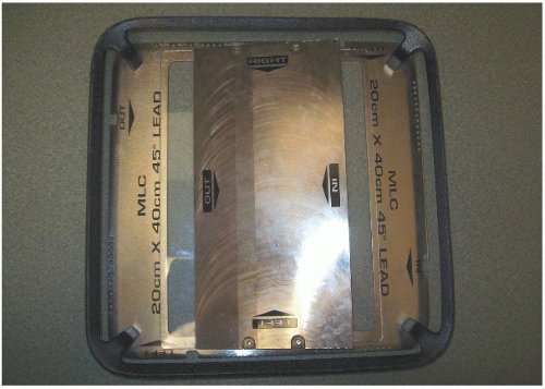Figure 11.7. Photograph of a 45-degree wedge filter (Varian 21 EX linac).

B. WEDGE ISODOSE ANGLE

The term wedge isodose angle (or simply wedge angle) refers to “the angle through which an isodose curve is titled at the central ray of a beam at a specified depth” (5). In this definition, one should note that the wedge angle is the angle between the isodose curve and the normal to the central axis, as shown in Figure 11.6. In addition, the specification of depth is important since, in general, the presence of scattered radiation causes the angle of isodose tilt to decrease with increasing depth in the phantom. The ICRU recommendation is to use a reference depth of 10 cm for wedge angle specification (5).

C. WEDGE TRANSMISSION FACTOR

The presence of a wedge filter decreases the output of the machine, which must be taken into account in treatment calculations. This effect is characterized by the wedge transmission factor (or simply wedge factor), defined as the ratio of doses with and without the wedge, at a point in phantom along the central axis of the beam. This factor should be measured in phantom at a suitable depth beyond the depth of maximum dose (e.g., 10 cm).

In cobalt-60 teletherapy, the wedge factor is sometimes incorporated into the isodose curves, as shown in Figure 11.6B. In this case, the depth dose distribution is normalized relative to the D_max without the wedge. For example, the isodose curve at depth of D_max is 72%, indicating that the wedge factor is already taken into account in the isodose distribution. If such a chart is used for isodose planning, no further correction should be applied to the output. In other words, the machine output corresponding to the open beam should be used.

A more common (and recommended) approach is to normalize the isodose curves relative to the central axis D_max with the wedge in the beam. As see in Figure 11.6A, the 100% dose is indicated at the depth of D_max. With this approach, the output of the beam must be corrected using the wedge factor.

D. PHYSICAL WEDGE SYSTEMS

Physical wedge filters are of two main types. The first may be called the individualized wedge system, which requires a separate wedge for each beam width, optimally designed to minimize the loss of beam output. A mechanism is provided to align the thin end of the wedge with the border of the light field (Fig. 11.8A). The second system uses a universal wedge; that is, a single wedge serves for all beam widths. Such a filter is fixed centrally in the beam, while the field can be opened to any size. As illustrated in Figure 11.8B

Only gold members can continue reading. Log In or Register to continue