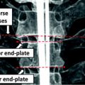
Vertebrae Localization and Labeling Using Learning-Based Approaches

Fig. 1

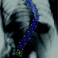
Challenges of vertebrae labeling in clinical cases. a A MR scan of a scoliosis patient. b A CT scan of a scoliosis patient. c A MR scan with folding artifact. d A CT scan with metal implant

In this chapter, we introduce a spine detection method that is highly robust to severe imaging artifacts and spine diseases. In principle, our method also use machine learning technologies to capture the appearance and geometry characteristics of spine anatomies. Similar to [11, 13, 15], i.e., low-level appearance and high-level geometry information are combined to derive spine detection. In particular, our method leverages two unique characteristics of spine anatomies. First, although a spine seems to be composed by a set of repetitive components (vertebrae and discs), these components indeed have different distinctiveness. Hence, different anatomies provide different levels of reliability and should be employed hierarchically in spine detection. Second, spine is a non–rigid structure, in which local articulations exist in-between vertebrae and discs. This kind of articulation can be quite large in the presence of certain spine diseases, e.g., scoliosis. An effective geometry modeling should not consider vertebrae detections from scoliotic cases as errors just because of the abnormal geometry.

Our method includes two strategies to leverage these two characteristics effectively. First, instead of learning a general detector for vertebrae/discs, we use a hierarchical strategy to learn detectors for anchor vertebrae, bundle vertebrae and inter-vertebral discs, respectively. Specifically, different learning strategies are designed to learn anchor, bundle and disc detectors considering different levels of “distinctiveness” of these anatomies. At run-time, these detectors are invoked in a hierarchial way. Second, a local articulation model is designed to describe spine geometries. It is employed to fuse the responses from hierarchical detectors. As the local articulation model satisfies the intrinsic geometric characteristics of both health and disease spines, it is able to propagate information from different detectors in a way that is robust to abnormal spine geometry. With the hallmarks of hierarchical learning and local articulated model, our method becomes highly robust to severe imaging artifacts and spine diseases.

3 Problem Statement

Notations: Human spine usually consists of 24 articulated vertebrae, which can be grouped as cervical ( $C_{1}$ – $C_{7}$ ), thoracic ( $T_{1}$ – $T_{12}$ ) and lumbar ( $L_{1}$ – $L_{5}$ ) sections. These 24 vertebrae plus the fused sacral vertebra ( $S_{1}$ ) are the targets of spine labeling in our study.

We define vertebrae and inter-vertebral discs as $V = \{ v_{i} |i = 1 \ldots N\}$ and $D = \{ d_{i} |i = 1 \ldots N - 1\}$ , where $v_{i}$ is the i-th vertebra and $d_{i}$ is the inter-vertebral disc between the i-th and i + 1-th vertebra. Here, $v_{i} \in {\mathbb{R}}^{3}$ is the vertebra center and $d_{i} \in {\mathbb{R}}^{9}$ includes the center, orientation and size of the disc. It is worth noting that

is not a simple index but bears anatomical definition. In this paper, without loss of generality, $v_{i}$ is indexed in the order of vertebrae from head to feet, e.g., $v_{1}$ , $v_{24}$ , $v_{25}$ represents $C_{1}$ , $L_{5}$ and $S_{1}$ , respectively.

Formulation: Given an image

, spine detection problem can be formulated as the maximization of a posterior probability with respect to

and

as:

$(V^{*} ,D^{*} ) = \arg \mathop {\hbox{max} }\limits_{V,D} P(V,D|I)$

(1)

Certain vertebrae that appear either at the extremity of the entire vertebrae column, e.g., $C_{2}$ , $S_{1}$ , or at the transition regions of different vertebral sections, e.g., $L_{1}$ , have much better distinguishable characteristics (red ones in Fig. 2a). The identification of these vertebrae helps in the labeling of others, and are defined as “anchor vertebrae”. The remaining vertebrae (blue ones in Fig. 2a) are grouped into a set of continuous “bundles” and hence defined as “bundle vertebrae”. Vertebrae characteristics are different across bundles but similar within a bundle, e.g., $C_{3}$ – $C_{7}$ look similar but are very distinguishable from $T_{8}$ – $T_{12}$ .

Fig. 2

a Schematic explanation of anchor (red) and bundle (blue) vertebrae. b Proposed spine detection framework

Denoting $V_{{\mathcal{A}}}$ and $V_{{\mathcal{B}}}$ as anchor and bundle vertebrae, the posterior in Eq. (1) can be rewritten and further expanded as:

$P(V,D|I) = P(V_{{\mathcal{A}}} ,V_{{\mathcal{B}}} ,D|I) = P(V_{{\mathcal{A}}} |I) \cdot P(V_{{\mathcal{B}}} |V_{{\mathcal{A}}} ,I) \cdot P(D|V_{{\mathcal{A}}} ,V_{{\mathcal{B}}} ,I)$

(2)

In this study, we use Gibbs distributions to model the probabilities. The logarithm Eq. (2) can be then derived as Eq. (3).

$\begin{array}{*{20}l} {\log [P(V,D|I)] = } & {A_{1} (V_{{\mathcal{A}}} |I)} \hfill & { \Leftarrow P(V_{{\mathcal{A}}} |I)} \hfill \\ {} & { +\, A_{2} (V_{{\mathcal{B}}} |I) + S_{1} (V_{{\mathcal{B}}} |V_{{\mathcal{A}}} )} \hfill & { \Leftarrow P(V_{{\mathcal{B}}} |V_{{\mathcal{A}}} ,I)} \hfill \\ {} & { +\, A_{3} (D|I) + S_{2} (D|V_{{\mathcal{A}}} ,V_{{\mathcal{B}}} )} \hfill & { \Leftarrow P(D|V_{{\mathcal{A}}} ,V_{{\mathcal{B}}} ,I)} \hfill \\ \end{array}$

(3)

Here, $A_{1}$ , $A_{2}$ and $A_{3}$ relate to the appearance characteristics of anchor, bundle vertebrae and inter-vertebral discs. $S_{1}$ and $S_{2}$ describe the spatial relations of anchor-bundle vertebrae and vertebrae-disc, respectively. It is worth noting that the posterior of anchor vertebrae solely depends on the appearance term, while those of bundle vertebrae and inter-vertebral discs depend on both appearance and spatial relations. This is in accordance to the intuition: while anchor vertebrae can be identified based on its distinctive appearance, bundle vertebrae and inter-vertebral discs have to be identified using both appearance characteristics and the spatial relations to anchor ones.

Figure 2b gives a schematic explanation of Eq. (3). Our framework consists of three layers of appearance models targeting to anchor, bundle vertebrae and discs. The spatial relations across different anatomies “bridge” different layers (lines in Fig. 2). Note that this framework is completely different from the two-level model of [11], which separates pixel- and object-level information. Instead, different layers of our framework target to anatomies with different appearance distinctiveness.

4 Hierarchical Learning Framework

4.1 Learning-Based Anatomy Detection

Before detailing hierarchical learning framework, we first introduce the basic learning modules for anatomy detection. Due to the complex appearance of vertebrae and discs, particularly in MR images, we resort to learning-based approach to model the appearance characteristics of vertebrae and inter-vertebral discs. Thanks to its data-driven nature, learning-based approaches also provide the scalability to extend our method on both CT and MR images. We formulate anatomy detection as a voxel-wise classification problem. Specifically, voxels within the anatomy primitive, i.e., vertebrae or inter-vertebral discs, are considered as positive samples and voxels away from the anatomy primitive are regarded as negative samples. To learn an anatomy detector, we first annotate vertebrae and inter-vertebral discs in training images. For each training sample (voxel), a set of elementary features are extracted in its neighborhood. Our elementary features are generated by a set of mother functions, $\{ H_{l} ({\mathbf{x}})\}$ extended from Haar wavelet basis. As shown in Eq. (4) and Fig. 3, each mother function consists of one or more 3D rectangle functions with different polarities.

Fig. 3

Some examples of haar-based mother functions

$H({\mathbf{x}}) = \sum\limits_{i = 1}^{N} p_{i} R({\mathbf{x}} - {\mathbf{a}}_{{\mathbf{i}}} )$

(4)

where polarities $p_{i} = \{ - 1,1\}$ , $$$R({\mathbf{x}}) = \left\{ {\begin{array}{*{20}l} {1,} \hfill & {{\kern 1pt} {\parallel }{\mathbf{x}}{\parallel }_{\infty } \le 1{\kern 1pt} } \hfill \\ {0,} \hfill & {{\kern 1pt} {\parallel }{\mathbf{x}}{\parallel }_{\infty } > 1{\kern 1pt} } \hfill \\ \end{array} } \right.$$” src=”/wp-content/uploads/2016/12/A312884_1_En_9_Chapter_IEq41.gif”></SPAN> denotes rectangle functions and <SPAN id=IEq42 class=InlineEquation><IMG alt=$${\mathbf{a}}_{{\mathbf{i}}}$$ src=$ is the translation.

By scaling the mother functions and convoluting them with the original image, a set of spatial-frequency spaces are constructed as Eq. (5).

$F_{l} ({\mathbf{x}},s) = H_{l} (s{\mathbf{x}})*I({\mathbf{x}})$

(5)

where

and

denote the scaling factor and index of mother functions, respectively.

Finally, for any voxel ${\mathbf{x}}_{{\mathbf{0}}} \in {\Re }^{\text{3}}$ , its feature vector ${\mathfrak{F}}({\mathbf{x}}_{{\mathbf{0}}} )$ is obtained by sampling these spatial-frequency spaces in the neighborhood of ${\mathbf{x}}_{{\mathbf{0}}}$ (Eq. 6). It provides cross-scale appearance descriptions of voxel ${\mathbf{x}}_{{\mathbf{0}}}$ .

${\mathfrak{F}}({\mathbf{x}}_{{\mathbf{0}}} ) = \bigcup\limits_{l = 1 \ldots L} \{ F_{l} ({\mathbf{x}}_{{\mathbf{i}}} ,s_{j} )|{\mathbf{x}}_{{\mathbf{i}}} \in {\mathbb{N}}({\mathbf{x}}_{{\mathbf{0}}} ),s_{ \hbox{min} } < s_{j} < s_{ \hbox{max} } \}$

(6)

Compared to standard Haar wavelet, the mother functions we employed are not orthogonal. However, they provide more comprehensive image features to characterize different anatomy primitives. For example, as shown in Fig. 3, mother function (a) potentially works as a smoothing filter, which is able to extract regional features. Mother functions (b) and (c) can generate horizontal or vertical “edgeness” responses, which are robust to local noises. More complicated mother function like (d) is able to detect “L-shape” patterns, which might be useful to distinguish some anatomy primitives. In addition, our features can be quickly calculated through integral image [21]. It paves the way to an efficient anatomy detection system.

All elementary features are then fed into a cascade classification framework [22] as shown in Fig. 4. The cascade framework is designed to address the highly unbalanced positive and negative samples. In fact, since only voxels around vertebrae centers or intervertebral discs are positives, the ratio of positives to negatives is often less than 1:10⁵. In the training stage, all positives but a small proportion of negatives are used at every cascade level. The training algorithm is “biased” to positives, such that each positive have to be correctly classified but the negatives are allowed to be misclassified. These misclassified negatives i.e., False Positives, will be further trained in the following cascades. At run-time, while positives will go through all cascades, most negatives can be rejected in the first several cascades and do no need further evaluation. In this way, the run-time speed can be dramatically increased. In our study, we use Adaboost [23] as the basic classifier in the cascade framework. The output of the learned classifier ${\mathcal{A}}({\mathfrak{F}}({\mathbf{x}}))$ indicates the existence likelihood of a landmark at ${\mathbf{x}}$ .

Fig. 4

Schematic explanation of cascade Adaboost classifers

Our learning-based framework is general to detect different anatomical structures in different imaging modalities due to two reasons. (1) The extended Haar wavelet generates thousands of features. In this large feature pool, there are always some features that are distinctive to specific anatomies. (2) The cascade learning framework is able to select the most distinctive features for a specific anatomy in a specific imaging modality.

In spine detection, a straightforward way to use this general detection framework is to train detectors for each vertebrae independently. However, these trained detectors might be confused by the similar appearances of neighboring vertebrae, particularly in the presence of diseases or imaging artifacts. An alternative way is to train a general detector to all vertebrae. However, due to the large shape and appearance variability across different vertebrae, e.g., the shape and size of cervical vertebrae are very different from lumbar vertebrae, it is very different to capture the common characteristics of all vertebrae with one detector/classifier. By observing these two limitations, we design a hierarchical learning scheme, which essentially categorize vertebrae and discs into different groups and use different training strategies based on their different characteristics. Specifically, our learning scheme consists of three layers, anchor vertebrae, bundle vertebrae and inter-vertebral discs.

4.2 Anchor Vertebrae

Anchor vertebrae (red ones in Fig. 2a) are vertebrae with distinctive characteristics. They are usually the vertebrae located at the extremes of vertebral column (e.g., C2, S1) or at the transition border of different spine sections (e.g., C7, L1). In radiology practices, anchor vertebrae usually provide critical evidences for labels of other vertebrae. To leverage the distinctive characteristics of anchor vertebrae, we build anchor vertebrae detectors as the first layer of our hierarchical learning scheme. The learning scheme is designed to achieve two goals. First, since anchor vertebrae have distinctive characteristics and can be identified exclusively, the detectors of anchor vertebrae should be very discriminative and only have high responses around the specific vertebrae centers. Second, as anchor vertebrae will be used to derive the labels of other vertebrae, the detection of anchor vertebrae should be highly robust.

To achieve the first goal, we train anchor vertebra detectors in a very discriminative way. Specifically, we only select voxels close to the specific anchor vertebra as the positives and all others are treated as negatives. Although the numbers of positive and negative samples become highly balanced, thanks to the cascade learning framework, we can still learn a discriminative detector for each anchor vertebra. To reach the second goal, for each anchor vertebrae, we define a set of “supporting landmarks” surrounding it. For example, for S1 vertebra, we use tip of coccyx, center of sacrum and spinous process of L5, etc., as its supporting landmarks. The strong spatial correlation between the supporting landmarks and the anchor vertebra are exploited to achieve robust detection. Mathematically, we employ a linear model to capture the spatial correlation between the anchor vertebra $v_{i}$ and its supporting landmarks ${\mathcal{S}}(v_{i} )$ as Eq. (7):

$\nu_{i} = {\mathfrak{C}} \cdot {\mathbb{U}}$

(7)

Here, ${\mathbb{U}}$ is a vector concatenated by coordinates of supporting landmarks and ${\mathfrak{C}}$ denotes the linear correlation matrix. Given a set of training samples, ${\mathfrak{C}}$ can be learned by solving a least squares problem. At run-time, besides detecting anchor vertebrae, we also detect its supporting landmarks. The learned linear correlation matrix are then used to verify the detected anchor vertebrae. In principle, we resort to “redundancy” [24] for highly robust anchor vertebrae detection.

4.3 Bundle Vertebrae

Different from anchor vertebrae, other vertebrae have less distinctive shapes and appearances. These vertebrae look similar to their neighbors but different from remote ones. On one hand, training a general detector for all bundle vertebrae is almost infeasible due to the large variations across distal ones. On the other hand, an attempt to learn the subtle differences between a bundle vertebra and its neighborhoods also adversely affects the robustness. For example, $T_{9}$ and $T_{10}$ are two neighboring vertebrae with similar appearance and shape characteristics. For normal cases (see Fig. 5a), the two detectors are still possible to distinguish the subtle differences between $T_{9}$ and $T_{10}$ . However, when the appearance of $T_{9}$ becomes abnormal due to imaging artifacts or diseases, $T_{9}$ detector might have higher responses at $T_{10}$ than $T_{9}$ (Fig. 5b), which induces wrong/miss labeled vertebrae. In fact, this problem is also observed in [15], where “(standard) MSL approach may end up with detections for the most salient disks only”.