3 Computed Tomography
Introduction
In computed tomography (CT) imaging, the X-ray tube and detector array rotate around the patient in a fixed geometry generating thousands of attenuation measurements through the patient volume of interest. The attenuation measurements are reconstructed into axial images which can then be reformatted into sagittal and coronal planes. The grayscale value displayed in each pixel represents the CT number in Hounsfield units of the corresponding voxel volume. CT number is a normalized measurement of the linear attenuation coefficient measured in the voxel relative to that of water, defined to be zero in value. As such, tissues that are more attenuating than water will have positive values in a CT image, and tissues that are less attenuating than water will have negative values. Each type of tissue in a CT image has a specific Hounsfield unit range which may be used quantitatively to characterize tissues or pathology.
Image quality in CT is affected by many parameters, some of which are selected by the operator prior to the acquisition, while others are selected prior to reconstruction of the data into tomographic planes. The same acquisition data can, therefore, be reconstructed in multiple ways to achieve different image quality end points dependent upon the clinical goals of the study.
3.1 Case 1: Ring Artifact
3.1.1 Background
Patient with a history of nephrolithiasis presented for CT of abdomen and pelvis examination.
A helical acquisition was acquired using a detector configuration of 24 × 1.2 mm channels.
Axial images of 3.0 mm thickness were reconstructed using a soft-tissue filter.
3.1.2 Findings
A partial ring artifact is centrally located in all axial reconstructions.
3.1.3 Discussion
The X-ray tube and detector array rotate around the CT gantry in a fixed geometry. The detector array consists of multiple detector channels in the z-direction, each containing many hundreds of individual detector elements in the x/y direction (Fig. 3‑1 b). 1 Each detector within the array measures the residual X-ray signal through the patient. If an individual detector within the array is not properly calibrated with respect to the other detectors, or fails completely, artifacts will appear in the reconstructed images. In helical acquisitions, the artifact will appear as a partial ring (Fig. 3‑1 a) and appear to rotate around isocenter throughout the imaging volume. Full ring artifacts will be present in axial scan acquisitions (Fig. 3‑1 c). The artifact will be limited to the images corresponding to the affected detector channel. For example, if a 16-channel system has a defective detector in channel 1, a full ring artifact will appear in the first reconstructed image and then again in image 17 but will not appear in images 2 to 16, assuming the width of the reconstructed slice is equal to the width of the detector channel.

3.1.4 Resolution
Axial acquisitions of a uniform water phantom, reconstructed at the thinnest possible slice thickness, should be acquired and evaluated for ring artifacts by the CT technologist on a daily basis. 2 When ring artifacts are identified, some CT systems will provide the user a method to recalibrate the detectors (often called an air calibration scan). If the air calibration scan is not available, or does not resolve the ring artifact, service personnel should be contacted and corrective maintenance be performed.
3.2 Case 2: Effect of Patient Size on CT Number Accuracy
3.2.1 Background
Bariatric patient with a history of renal calculi presents with abdominal pain.
A helical abdomen/pelvis CT is performed.
Incidental finding in the adrenal gland with elevated CT number measurement.
3.2.2 Findings
Use of CT number for quantitative analysis can be compromised in bariatric patients due to beam hardening and truncation artifact.
3.2.3 Discussion
The X-ray tube used in CT produces a polyenergetic X-ray beam. Filters are placed at the exit port of the beam to remove low-energy X-rays increasing the average energy of the X-ray beam. A process called beam hardening. As the X-ray beam enters the patient, beam hardening continues as the lower-energy X-rays in the beam are attenuated with higher probability. The displayed CT number is a relative measure of attenuation as compared to the attenuation of water. As the beam becomes more energetic (hardened), less attenuation occurs in a given tissue which changes the CT number. In a typically sized patient, this beam hardening effect is corrected for by the scanner. In bariatric patients, the beam hardening effect is more significant and can affect the accuracy of displayed CT numbers. When the patient’s tissues fall outside of the scan field of view (FOV), the system overestimates the attenuation provided by the tissues within the FOV. This is often referred to as a truncation artifact and appears as bright areas in the image (Fig. 3‑2 a). Truncation artifact can also affect the accuracy of CT numbers used for quantitative analysis. 3

3.2.4 Resolution
Some systems may offer an extended FOV reconstruction option as shown in Fig. 3‑2 b. In this case, the visual appearance of the truncation artifact was reduced by reconstructing using an extended FOV; however, little effect on measured CT number in the adrenal gland was realized. Patient positioning can also have a significant impact on beam hardening and truncation artifacts in bariatric patients. The patient in this case, presented for another scan 2 weeks later (Fig. 3‑2). Note the difference in the patient’s apparent shape and diameter. This was due to more effective wrapping of extraneous tissues by the technologist prior to scanning and is not related to patient weight loss. No truncation artifact is present and the change in measured Hounsfield units is significant.
3.3 Case 3: Effect of kV Selection on Image Quality and Dose
3.3.1 Background
Patient with a history of cecal and appendiceal adenocarcinoma with multiple prior CT examinations presents for chest/abdomen/pelvis CT with contrast post resection with peroneal nodules for evaluation of treatment.
A helical acquisition is acquired at reduced kV compared to prior studies.
3.3.2 Findings
Contrast is improved at the lower kV setting at a dose savings of approximately 17%.
3.3.3 Discussion
Lowering tube voltage (kV) produces an X-ray beam with lower average and maximum energy. Lower X-ray energies will be attenuated in a given tissue more than higher-energy X-rays. This is primarily governed by differences in attenuation that occurs due to photoelectric absorption which is approximately proportional to the atomic number (Z) cubed of the tissue, and inversely proportional to the energy (E) cubed of the X-ray beam. As such, the relative attenuation between two tissues increases at lower kV settings. On a CT image, this results in a greater difference in Hounsfield units between the two tissues, and therefore, greater contrast. Note the increased contrast of the seminal vesicle structure shown in Fig. 3‑3 a which was acquired at 100 kV as compared to the same structure in Fig. 3‑3 b acquired at 120 kV.

Tube voltage (kV) also affects the efficiency of X-ray production in the X-ray tube. At a lower kV setting, the number of X-rays produced is reduced by the ratio of the change in kV squared to cubed (∆kV2–3). Quantum noise increases when fewer X-rays are used to make the image, which will have a negative effect on the visibility of low-contrast structures. To compensate, a decrease in kV is often accompanied by an increase in tube current (mA). As shown in Fig. 3‑3 a, b, an appropriate increase in mA to achieve an acceptable level of quantum noise levels can be achieved at a significant dose reduction.
3.3.4 Resolution
Tube voltage and current settings should be adjusted to optimize image quality and dose. The usefulness of this technique will depend on patient size and the anatomy/pathology of interest. A lower kV setting can often be used on smaller patients. In very large patients, the mA limitations of the X-ray tube may result in increased photon starvation artifacts. Beam hardening artifacts will also be enhanced at low kV settings. Lower-energy beams are also effective when using iodinated contrast agents as the average beam energy more closely aligns with the k-edge absorption peak of iodine. Care should be taken when using CT numbers for quantitative analysis as the CT number is affected by the kV setting.
3.4 Case 4: Image Quality Variation with Reconstructed Slice Thickness
3.4.1 Background
Patient presents to the emergency department following a motor vehicle collision.
CT thorax, CT abdomen, and pelvis examinations following the administration of contrast were acquired.
Axial images of 3.0 and 1.5 mm slice thickness were reconstructed.
3.4.2 Findings
Small fracture of the clavicle is not visible with 3.0 mm reconstructed slices.
3.4.3 Discussion
Reconstructed slice thickness affects the level of quantum noise, spatial resolution, and partial volume averaging present in CT images. Slice thickness affects the size of the reconstructed tissue voxel. Each voxel of tissue is displayed as one shade of gray in the corresponding image pixel. When the voxel contains more than one type of tissue or pathology, the CT number displayed represents the average attenuation measurement of all the tissues within the voxel. This principle is called partial volume averaging and is inherent to the CT image reconstruction process. As the tissue voxel becomes larger and there is more signal averaging, there is less spatial differentiation of the signal in a given direction and the image appears more blurred, with lower spatial resolution. Fig. 3‑4 a is reconstructed with a 1.5 mm slice thickness and Fig. 3‑4 b is reconstructed with a 3.0 mm slice thickness. The thinner reconstructions are sharper (better spatial resolution) and have less partial volume averaging. Note the subtle clavicle fracture seen on the 1.5-mm reconstructions which is not visible on the 3.0-mm reconstructions. Quantum noise is also affected by the size of the reconstructed voxel. The amount of signal (number of X-rays) interacting within a given voxel is directly proportional to voxel size. Quantum noise changes inversely with the square root of the change in signal.

3.4.4 Resolution
Voxel size is a function of the pixel size and the reconstructed slice thickness selected by the operator. When reconstructed slice thickness is increased, more partial volume averaging occurs in the slice thickness direction. When a thinner reconstructed slice thickness is selected, there is better differentiation of tissues along the slice thickness direction resulting in better spatial resolution and less partial volume averaging. CT protocols often include multiple reconstructions of the same acquisition at different reconstructed slice thicknesses to provide the clinician with high spatial resolution image series as well as low noise image series for evaluation.
The only other parameter that affects the size of the reconstructed voxel in CT is the FOV selected by the operator prior to reconstruction. FOV is often selected to encompass the anatomy of interest and determines the size of the tissue voxel and corresponding image pixel in the x and y dimension.
3.5 Case 5: Image Quality Variation with Reconstruction Filter
3.5.1 Background
Patient with a history of bacterial meningitis and multiple brain abscesses presents for follow-up CT to evaluate the response to treatment with IV antibiotics.
Helical CT of the head is acquired with contrast and reconstructed using filtered back projection.
A reduced mA technique is implemented in an effort to reduce patient radiation dose.
Related posts:

Stay updated, free articles. Join our Telegram channel

Full access? Get Clinical Tree


