Fig. 1
Examples of lytic and sclerotic metastases in the spine. First row lytic metastases. Second row sclerotic metastases
2 Background of Computer Aided Detection
Detection of spinal metastases on CT can be a challenge, as the spinal column is a physically extended and complex structure. Lesion presentation may be subtle and unexpected. Adding to this complexity, in the current clinical practice environment, multiple high-throughput CT scanners can produce numerous patient studies in a short time interval, each with thousands of images, restricting time for image assessment. Numerous anatomic structures in each image must be assessed for pathology, typically at multiple window/level settings, effectively increasing the number of images to be reviewed geometrically.
Computer Aided Detection (CAD) researchers have been active in the past two decades and have showed very promising results. CAD is a potential solution to the challenge of rapid assessment of very large datasets. CAD is a software tool that can detect, mark, and quantitatively assess potential pathologies for further scrutiny by a radiologist. The CAD system should be topically focused with the ability to facilitate rapid and accurate assessment of important anatomy or high risk pathology subsets of interest in the CT data, such as the spine. While the final diagnosis is made by the radiologist responsible for interpreting the examination, CAD can help improve sensitivity in identifying lesions potentially overlooked by radiologists in situations of data overload or fatigue.
Figure 2 is a block diagram of a typical CAD system. A typical CAD system has two phases: training and testing. In the training phase, a set of training data is first collected. Then radiologist’s diagnostic knowledge is applied to analyze the training data and to derive detection rules (classifiers). In the testing phase, clinical images are taken as input. An image segmentation step is performed to extract structures of interest and limit the search region. Characteristic features of the structures are computed. Relevant features are then selected and input into a classifier. With the aid of the detection rules developed in the training phase, the classifier distinguishes true lesions from false lesions, or malign lesions from benign lesions. The preliminary detections are then reported to radiologists for final decisions.
Fig. 2
Block diagram of computer aided detection
Characteristic features for classification include features traditionally used by radiologists and high-order features that are not inherently intuitive. Features include shape features such as circularity, sphericity, compactness, irregularity, elongation, or density features such as contrast, roughness, and texture attributes. Different detection tasks need different sets of relevant features. Feature selection techniques, such as forward stepwise method and genetic algorithm, are applied in the training phase to choose features for further classification [20]. Several classifiers have been proposed for different applications, including linear discriminant analysis, Bayesian methods, artificial neural network, and support vector machine [21].
The quality of a CAD system can be characterized by the sensitivity and specificity of the system detection. Sensitivity refers to the fraction of diseased cases correctly identified as positive in the system (true positive fraction, TPF). Specificity refers to the fraction of disease-free cases correctly identified as negative. “Receiver operating characteristic” (ROC) curves are used to describe the relationship between sensitivity and specificity. The ROC curves show the true-positive fraction (TPF = sensitivity) versus the false-positive fraction (FPF = 1 − specificity). In addition to ROC curves, Free-response ROC (FROC) curves (TPF versus false positive per case) were proposed to more accurately represent the number of false positive detections [22]. The areas under the ROC and FROC curve are measures of the quality of a CAD system. There is often a tradeoff between achieving high specificity and high sensitivity. A successful CAD system should detect as many true lesions as possible while minimizing the false positive detection rate.
CAD systems have been used to detect lesions in the breast, where the increased the true positive rate in breast cancer screening and improved the yield of biopsy recommendations for patients with masses on serial mammograms [23, 24]. CAD has been shown to improve radiologists’ performance detecting lung nodules on chest radiography and CT [25, 26] and to increase sensitivity for detecting polyps on CT colonography [27]. In spine imaging, CAD systems had been developed to detect spine abnormality and disease such as lytic lesions [28], sclerotic lesion [29], fractures [30], degenerative disease [31], syndesmophyte [32] and epidural masses [33]. Several commercial systems in mammography, chest CT and CT colonography have already received FDA approval for clinical use.
CAD involves all aspects of medical image processing techniques. For instance, image segmentation and registration are necessary for feature computation, and image visualization and measurement are essential to present the results to clinicians.
3 Spine Metastasis CAD System Overview
Bone metastases can appear lytic, sclerotic, or anywhere in a continuum between these extremes. Therefore, automated detection of these lesions is a complex problem that must be broken down into manageable components. We develop a CAD framework that can handle both types of bone metastases. The CAD system is a supervised machine learning framework. By supplying the CAD system with different sets of labeled training data for lytic and sclerotic bone metastases, we can train the system to detect the two types of bone metastases separately. The framework has two phases: training phase and testing phase. Training phase has four stages: spine segmentation, candidate detection, feature extraction and classifier training. The testing stage also has four stages: spine segmentation, candidate detection, feature extraction and classification. The first three stages of training and testing phases are identical. The training phase is an offline process and can be fine-tuned by researchers, and the testing phase is fully automatic. Each stage will be elaborated upon in the following sections.
4 Spinal Column Segmentation and Partitioning
Spine is a bony structure with higher CT value (pixel intensity) than other tissue types. The CT value is a gauge of X-ray beam attenuation measured by the CT scanner, and historically was normalized into a standardized scaling set referred to as Hounsfield units (HU). We first apply a threshold of 200 HU to mask out the bone pixels. Then a connected component analysis is conducted on the bone mask and the largest connected component in the center of the image is retained as the initial spine segmentation. The bounding box of the initial segmentation is used as the search region for the following segmentation tasks.
The spinal canal links all vertebrae into a column. On a transverse cross section, the spinal canal appears as a low intensity oval region surrounded by high density pedicle and lamina (Fig. 3a). The extraction of the spinal canal is essential in order to accurately localize the spine and form the spinal column. We apply a watershed algorithm to detect the potential spinal canal regions, and then conduct a graph search to locate and extract the spinal canal.
Fig. 3
Spinal canal extraction. a CT image; b watershed result; c spinal canal candidates; d directed acyclic graph (DAG), number on the edge is the weight between two nodes; and e extracted spinal canal (blue color)
The principle of the watershed algorithm [34] is to transform the gradient of a gray level image into a topographic surface. The algorithm simulates the watershed scenario by puncturing holes at the local minimum of the intensity and filling the region with water. Each region filling with water is called a catchment basin. The spinal canal resembles a catchment basin on a 2D cross sectional image. We adopted the watershed algorithm implementation in ITK [35].
The well-known over-segmentation problem of the watershed algorithm is alleviated by merging adjacent basins. Depth of a basin is defined in Eq. 1.
here I(x) is the image intensity of a pixel x inside the basin b. Given a and b are two neighboring basins, they will be merged if both conditions in Eq. 2 are satisfied
here N(a) denotes neighbors of basin a, δ m is the merging threshold. After that, all basins that meet the criteria in Eq. 3 and surrounded by bone pixels are recorded as potential candidates for the spinal canal.
![$$ d(c_{i} ) - d(b) > \delta_{d} ,\quad \forall c_{i} \in N(b) $$” src=”/wp-content/uploads/2016/12/A312884_1_En_4_Chapter_Equ3.gif”></DIV></DIV><br />
<DIV class=EquationNumber>(3)</DIV></DIV>here <SPAN class=EmphasisTypeItalic>δ</SPAN> <SUB><SPAN class=EmphasisTypeItalic>d</SPAN> </SUB>is the depth contrast threshold. Figure <SPAN class=InternalRef><A href=]() 3b, c show the result of the watershed algorithm and the candidates for spinal canals.
3b, c show the result of the watershed algorithm and the candidates for spinal canals.
(1)
(2)
As showed in Fig. 3c, multiple canal candidates may exist in one slice due to the partial volume effect or loss density vertebra body region such as lytic bone lesion. We propose a method to extract the correct spinal canal using directed graph search. We first build a directed acyclic graph (DAG) from the canal candidates. The DAG is illustrated in Fig. 3d. The graph G(N, A) is a structure that consists of a set of nodes N and a set of directional edges E. A node is one canal candidate. A directional edge  connects two nodes n 1 and n 2 on adjacent slices, where the weight of
  is computed as the overlap of n 1 and n 2, as in Eq. 4.
connects two nodes n 1 and n 2 on adjacent slices, where the weight of is computed as the overlap of n 1 and n 2, as in Eq. 4.(4)
An edge only exists when its weight is greater than 0 (two nodes overlap). DAG has sources on the first slice and sinks on the last slice. A directed graph searching algorithm [36] is applied to find the longest path from source to sink, which is the spinal canal in our case. In Fig. 3d, the longest path is marked with red color. The centerline of the spinal canal is then computed and smoothed using a Bernstein spline [37]. Figure 3e shows the extracted spinal canal (blue color).
Vertebra segmentation is commonly implemented using geometric and statistical models owing to its articulated and complex structure (Fig. 4a) [38–40]. The anatomical models capture the shape, topology and inter-relationship of vertebrae, and therefore convert the image segmentation problem to a model fitting problem. We proposed a four-part vertebral model to segment the vertebral region on a 2D slice. The model includes four main vertebra sub-structures: vertebral body, posterior spinous process, left transverse process and right transverse process (see Fig. 4b). The vertebral body is modeled as a circle with a medial atom in the center and border atoms evenly distributed on the border. The spinous and transverse processes are modeled as slabs with a medial axis and a set of border atoms on each side. The model’s multiple-part structure simplifies the problem and makes the segmentation robust. Each model part is essentially a medial model [41]. The medial axis defines the skeleton, and the border atoms define the boundary.
Fig. 4
Spine segmentation. a Vertebra anatomical illustration; b vertebra template; c Initial template superimposed on CT; and d segmentation results
The border of the medial model can be written as an implicit function in the local coordinate of the model

(5)
A border atom A i can then be represented in the local coordinate, as A i = (u i , v i ) = (u i , f(u i )). In the coordinate system of the disk model, u is the radian angle around the center and v is the distance to the center. In the coordinate system of the slab model, u is the distance along the medial axis and v is the distance to the medial axis.
The segmentation task is to locate the border atoms so that a maximum model-to-image match can be reached. The matching metric should also preserve the model topology and border smoothness constraint. We design a metric for the model matching:
Here (u i , f(u i )) are the border atoms. The metric has four components, the directional gradient  is to match the border atoms with the intensity edge of the image,
  and
and  are smoothness constraints on the border, and p(u i , f(u i )) is a penalty function to prevent intersecting between model parts. Weights w g , w 1, w 2 and w p are set empirically.
(6)
is to match the border atoms with the intensity edge of the image, and are smoothness constraints on the border, and p(u i , f(u i )) is a penalty function to prevent intersecting between model parts. Weights w g , w 1, w 2 and w p are set empirically.The extracted spinal canal defines the initial location and size of the vertebra model. The model matching proceeds sequentially. First the vertebral body is matched, followed by the spinous process, and at the end the transverse processes. The results of the previous steps are used to determine the initial location and size of the parts in the following steps. In our current model, we define 36 border atoms for the disk model and 20 atoms for the slab models.
5 Spinal Column Partitioning
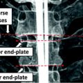
The spinal column consists of a set of vertebrae separated by inter-vertebral discs (Fig. 5a). Since the spinal column is a curved structure, the standard planar reformations (sagittal and coronal) do not provide clear views of the vertebral separation (Fig. 5b). Curved planar reformation (CPR) (Fig. 5c) [42] is generally considered superior.
Fig. 5
Spine partitioning. a Spinal column; b regular sagittal reformation; c curved planar reformation in sagittal direction; d aggregated intensity profile (AIP) along the spinal canal; e spinal partitioning in sagittal direction; f spine partition in coronal direction; and g spine partition in 3D, red planes are the partitioning planes
After the spinal column is segmented, we need to partition the spinal column into vertebrae at the inter-vertebral disc locations so that we can process the vertebrae separately and also localize the abnormality at the vertebra level. We developed a partitioning approach based on curved reformation along the spinal canal.
The centerline of the spinal canal is used as the central axis for the CPR. We generate the CPR in sagittal and coronal directions. Given that the vertices on the centerline are  , j = 1…n, the curved reformation in the sagittal direction is written as
where I Sag is the curved reformatted sagittal image, I 3D is the original 3D image. (x i , y i ) is the 2D coordinate in the reformatted image. Similarly, the curved reformation in the coronal direction is written as
where I Cor is the reformatted coronal image. Figure 5b, c show the regular coronal reformation, together with the curved planar reformation in sagittal and coronal directions. The curved reformations clearly better reveal the inter-vertebral disks.
, j = 1…n, the curved reformation in the sagittal direction is written as(7)
(8)
To make use of the CPR for spinal column partitioning, the centerline of the spinal canal is first projected onto the reformatted images. Then the normal is computed at every point on the centerline. The intensity along the normal direction is then aggregated and recorded. Figure 5d shows the aggregated intensity profile (AIP) along the spinal cord at the reformatted coronal view. As observed, the aggregated intensity at the disc location is lower than those at the vertebral body location. However, the difference is still not prominent, especially at cervical spine and highly curved region. We further convolve the aggregated intensity profile with an adaptive disk function, which can be written as,
![$$ f(x) = \left\{ {\begin{array}{*{20}l} { - 1} & {x \in [ - T/2,T/2]} \\ 1 & {Elsewhere} \\ \end{array} } \right. $$](/wp-content/uploads/2016/12/A312884_1_En_4_Chapter_Equ9.gif)
(9)
The function is a rectangle function with adaptive width T. In order to determine T, we search the neighborhood in both directions on the AIP for local maximum values.
The intervertebral disks are then located at the lowest response points on the adjusted intensity profile and used to partition the spinal column. Figure 5e, f show the spine partition superimposed on reformatted CPR views and the spinal column with vertebral partitions in a 3D view is shown in Fig. 5g.
6 Metastasis Candidate Detection
After the spine is segmented, the following lesion detection processes are restricted to the segmented spine excluding the spinal canal. We locate bone metastasis candidates in three steps. First a watershed algorithm is applied to extract initial super-pixels as metastasis candidates, followed by a merging routine based on graph cut to alleviate over-segmentation. The resulting 2-D candidates are then merged into 3-D detections. For each 3-D candidate, a set of features is computed and passed through a detection filter. The candidates which successfully pass through the detection filter are then sent to the next stage for classification.
The watershed algorithm is again applied to detect the metastasis candidates. Watershed algorithm views the gradient of the image intensity as a topographic surface in order to extract relatively homogeneous regions of the image called catchment basins, some of which will be candidates for lesions. The algorithm can be adapted for both lytic and sclerotic lesions. For lytic lesions, low intensity regions surrounded by high intensity regions are detected. Similarly, for sclerotic lesions, high intensity regions surrounded by low intensity regions are detected. Example results of the watershed algorithm are shown in Fig. 6.
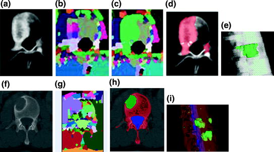
Fig. 6
Candidate detection and segmentation. a CT image of a vertebra with sclerotic lesions; b watershed result; c graph cut result after watershed; d candidate sclerotic lesions; e 3D segmented sclerotic lesions; f CT image of a vertebra with lytic lesions; g watershed result; h candidate lytic lesions; and i 3D segmented lytic lesions
We then address the over-segmentation problem in watershed with a post-watershed merging routine using a graph-cuts strategy [43]. Without loss of generality, we use the sclerotic lesion detection to describe the graph-cut strategy. We first initialize each watershed region with a foreground (F) or background (B) label. There are two types of foreground regions: those in the cortical bone region and those in the medullary regions. Any region that has intensity 100 HU higher than its surrounding regions (cortical or medullary) will be initialized as F. The rest of the regions are initialized as B. The regions and their neighbors are fed into a graph-cuts merging routine.
An adjacency graph for watershed regions is constructed by representing adjacent regions as nodes connected by edges [44]. The technique partitions the set of nodes into two disjoint sets F and B in a manner that minimizes an energy function,
where P is the set of watershed regions, N is the set of pairs of adjacent regions, L is a labeling of all the regions where a given region p can have the label L p = F or L p = B, V is a smoothness term that penalizes regions with similar densities having different labels, and D is a data term that penalizes a region with low density marked as foreground, or a region with high density marked as background. Thus the technique will merge higher-density regions into the foreground, and lower-density regions into the background. In this case,
where K F = 100, K B = 1 in our setting, I(p) is the mean intensity of region p, and m B and m F are the means of the background and foreground respectively. As for the smoothness term, we chose
where K s = (δ F + δ B )/2, δ F and δ B are the standard deviation of the foreground and background respectively.  are the cumulative histogram of region p, and
  .
.
(10)
(11)
(12)
are the cumulative histogram of region p, and .The smoothness and data penalty functions provide edge weights w(i, j) for a graph G consisting of the adjacency graph of the watershed regions and two additional nodes f and b which both have edges connecting them to every region node:

(13)
A graph cut [F, B] is a partition of the set of nodes such that  and
and  , and the value of the cut is,
and , and the value of the cut is,(14)
A minimal graph cut of G is equivalent to a labeling that minimizes Eq. (10). Such a cut is computed according to a max-flow algorithm referenced in which generates a local minimum within a known factor of the global minimum. The resulting partition [F, B] yields an optimized way of merging watershed regions in which regions corresponding to nodes in F and B are labeled as F and B respectively. Figure 6c demonstrates the effect of this merger. Each merged F region is then regarded as one potential detection.
So far, the candidates are all two-dimensional. Lesions actually extend through the spine in three dimensions. Therefore the next step is to merge the two-dimensional candidates that belong to the same lesion into a single three-dimensional “blob”. Two candidates A and B are merged if and only if
1.
They lie in adjacent slices z and z + 1
2.
For all 2-D candidates C on slice(z + 1) and all D on slice(z), it is true that
![$$ \begin{gathered} {{\left( {{{pr_{A} \left( B \right)} \mathord{\left/ {\vphantom {{pr_{A} \left( B \right)} {a\left( A \right)}}} \right. \kern-0pt} {a\left( A \right)}} + {{pr_{B} \left( A \right)} \mathord{\left/ {\vphantom {{pr_{B} \left( A \right)} {a\left( B \right)}}} \right. \kern-0pt} {a\left( B \right)}}} \right)} \mathord{\left/ {\vphantom {{\left( {{{pr_{A} \left( B \right)} \mathord{\left/ {\vphantom {{pr_{A} \left( B \right)} {a\left( A \right)}}} \right. \kern-0pt} {a\left( A \right)}} + {{pr_{B} \left( A \right)} \mathord{\left/ {\vphantom {{pr_{B} \left( A \right)} {a\left( B \right)}}} \right. \kern-0pt} {a\left( B \right)}}} \right)} 2}} \right. \kern-0pt} 2} > {{\left( {{{pr_{A} \left( C \right)} \mathord{\left/ {\vphantom {{pr_{A} \left( C \right)} {a\left( A \right)}}} \right. \kern-0pt} {a\left( A \right)}} + {{pr_{C} \left( A \right)} \mathord{\left/ {\vphantom {{pr_{C} \left( A \right)} {a\left( C \right)}}} \right. \kern-0pt} {a\left( C \right)}}} \right)} \mathord{\left/ {\vphantom {{\left( {{{pr_{A} \left( C \right)} \mathord{\left/ {\vphantom {{pr_{A} \left( C \right)} {a\left( A \right)}}} \right. \kern-0pt} {a\left( A \right)}} + {{pr_{C} \left( A \right)} \mathord{\left/ {\vphantom {{pr_{C} \left( A \right)} {a\left( C \right)}}} \right. \kern-0pt} {a\left( C \right)}}} \right)} 2}} \right. \kern-0pt} 2} \hfill \\ {\text{and}}\,{{\left( {{{pr_{A} \left( B \right)} \mathord{\left/ {\vphantom {{pr_{A} \left( B \right)} {a\left( A \right)}}} \right. \kern-0pt} {a\left( A \right)}} + {{pr_{B} \left( A \right)} \mathord{\left/ {\vphantom {{pr_{B} \left( A \right)} {a\left( B \right)}}} \right. \kern-0pt} {a\left( B \right)}}} \right)} \mathord{\left/ {\vphantom {{\left( {{{pr_{A} \left( B \right)} \mathord{\left/ {\vphantom {{pr_{A} \left( B \right)} {a\left( A \right)}}} \right. \kern-0pt} {a\left( A \right)}} + {{pr_{B} \left( A \right)} \mathord{\left/ {\vphantom {{pr_{B} \left( A \right)} {a\left( B \right)}}} \right. \kern-0pt} {a\left( B \right)}}} \right)} 2}} \right. \kern-0pt} 2} > {{\left( {{{pr_{D} \left( B \right)} \mathord{\left/ {\vphantom {{pr_{D} \left( B \right)} {a\left( D \right)}}} \right. \kern-0pt} {a\left( D \right)}} + pr_{B} \left( D \right)/a\left( B \right)} \right)} \mathord{\left/ {\vphantom {{\left( {{{pr_{D} \left( B \right)} \mathord{\left/ {\vphantom {{pr_{D} \left( B \right)} {a\left( D \right)}}} \right. \kern-0pt} {a\left( D \right)}} + pr_{B} \left( D \right)/a\left( B \right)} \right)} 2}} \right. \kern-0pt} 2}, \hfill \\ \end{gathered} $$” src=”/wp-content/uploads/2016/12/A312884_1_En_4_Chapter_Equa.gif”></DIV></DIV></DIV>where <SPAN class=EmphasisTypeItalic>slice</SPAN>(<SPAN class=EmphasisTypeItalic>z</SPAN>) is the CT slice at height <SPAN class=EmphasisTypeItalic>z</SPAN>, <SPAN class=EmphasisTypeItalic>pr</SPAN> <SUB><SPAN class=EmphasisTypeItalic>X</SPAN> </SUB>(<SPAN class=EmphasisTypeItalic>Y</SPAN>) is the fraction of candidate <SPAN class=EmphasisTypeItalic>Y</SPAN> that overlaps with <SPAN class=EmphasisTypeItalic>X</SPAN> when projected into the slice of <SPAN class=EmphasisTypeItalic>X</SPAN>, and <SPAN class=EmphasisTypeItalic>a</SPAN>(<SPAN class=EmphasisTypeItalic>X</SPAN>) is the area of candidate <SPAN class=EmphasisTypeItalic>X</SPAN>. In other words, the average projectional overlap of <SPAN class=EmphasisTypeItalic>A</SPAN> and <SPAN class=EmphasisTypeItalic>B</SPAN> is greater than the average projectional overlap of <SPAN class=EmphasisTypeItalic>A</SPAN> with any other candidate in the same slice as <SPAN class=EmphasisTypeItalic>B</SPAN>, and also greater than the average projectional overlap of <SPAN class=EmphasisTypeItalic>B</SPAN> with any candidate in the same slice as <SPAN class=EmphasisTypeItalic>A</SPAN>.</DIV></DIV><br />
<DIV class=ClearBoth> </DIV></DIV></DIV></DIV><br />
<DIV class=Para>After the lesions are detected in 3D, a level set algorithm is applied to obtain the 3D segmentation so that characteristic features can be derived. Level sets are evolving interfaces (contours or surfaces) that can expand, contract, and even split or merge. Level set methods are part of the family of segmentation algorithms that rely on the propagation of an approximate initial boundary under the influence of images forces [<CITE><A href=]() 45]. The underlying idea behind the level set method is to embed the moving interfaces as the zero level set of a higher dimensional function
45]. The underlying idea behind the level set method is to embed the moving interfaces as the zero level set of a higher dimensional function  , defined as

where  is the signed distance to the interface from point x. That is, x is outside the interface when
  , and on the interface when
  . The evolution of
  can be represented by a partial differential equation:
 Assistance and Intervention in Spine Surgery
 Ultrasound in Navigated Spine Interventions
 Column Localization, Labeling, and Segmentation
 Model-Based Vertebra Identification from X-Ray Image(s)
 Spine Reconstruction from Radiographs
 Segmentation, Reconstruction and Analysis of the Vertebral Body from Spinal CT


 Get Clinical Tree app for offline access

, defined as(15)
is the signed distance to the interface from point x. That is, x is outside the interface when , and on the interface when . The evolution of can be represented by a partial differential equation:Related posts:
Assistance and Intervention in Spine Surgery
Ultrasound in Navigated Spine Interventions
Model-Based Vertebra Identification from X-Ray Image(s)
Spine Reconstruction from Radiographs
Segmentation, Reconstruction and Analysis of the Vertebral Body from Spinal CT
Stay updated, free articles. Join our Telegram channel
Full access? Get Clinical Tree