and Lori Ann Lewis1
(1)
Clinical Research Center of North Texas, Denton, TX, USA
Abstract
In any discussion of bone densitometry, many terms and conventions are used that are unique to this field. In the chapters that follow, these terms and conventions will be used repeatedly. In an effort to facilitate the reading and comprehension of those chapters, a preliminary review of some of these unique aspects of bone densitometry is offered here.
In any discussion of bone densitometry, many terms and conventions are used that are unique to this field. In the chapters that follow, these terms and conventions will be used repeatedly. In an effort to facilitate the reading and comprehension of those chapters, a preliminary review of some of these unique aspects of bone densitometry is offered here.
Densitometry as a Quantitative Measurement Technique
Bone densitometry is primarily a quantitative measurement technique. That is, the technology is used to measure a quantity, in this case, the bone mass or density. Other quantitative measurement techniques used in clinical medicine are sphygmomanometry, spirometry, and the measurement of hemoglobin, cholesterol, glucose, and other substances found in the blood. Some of today’s highly sophisticated densitometers are capable of producing extraordinary skeletal images that may be used for structural diagnoses. Nevertheless, densitometry primarily remains a quantitative measurement technique, rather than an imaging technique like plain radiography. As such, quality control measures in densitometry are not only concerned with the mechanical operation of the devices, but with attributes of quantitative measurements such as accuracy and precision.
Accuracy and Precision
Accuracy and precision are easily understood using a target analogy shown in Fig. 1-1. To hit the bull’s-eye of the target is the goal of any archer. In a sense, the bull’s-eye is the gold standard for accuracy. In Fig. 1-1 on target A, one of the archer’s arrows has, in fact, hit the bull’s-eye. Three of the other four arrows are close to the bull’s-eye as well, although none has actually hit it. One arrow is above and to the right of the bull’s-eye in the second ring. A second arrow is to the right and below the bull’s-eye in the second ring, and a third arrow is below and to the left of the bull’s-eye straddling rings 1 and 2. The last arrow is straddling rings 2 and 3, above and to the left of the bull’s-eye. This archer can be said to be reasonably accurate, but he has been unable to reproduce his shot. Target A illustrates accuracy and lack of precision. In target B, another archer has attempted to hit the bull’s-eye. Unfortunately, he has not come close. He has, however, been extremely consistent in the placement of his five arrows. All five are tightly grouped together in the upper right quadrant of the target. In other words, although not accurate, this archer’s shots were extremely reproducible, or precise. Target B illustrates precision and lack of accuracy. Ideally, an archer would be both accurate and precise, as shown in target C in Fig. 1-1. Here all five arrows are grouped together within the bull’s-eye, indicating a high degree of both accuracy and precision.
Fig. 1-1.
Accuracy and precision. Target A illustrates accuracy without precision. Target B illustrates precision without accuracy. In target C, a high degree of both accuracy and precision is illustrated.
When bone densitometry is used to quantify the bone density for the purpose of diagnosing osteoporosis or predicting fracture risk, it is imperative that the measurement be accurate. On the other hand, when bone densitometry is used to follow changes in bone density over time, precision becomes paramount. Strictly speaking, the initial accuracy of the measurement is no longer of major concern. It is only necessary that the measurement be reproducible or precise since it is the change between measurements that is of interest. Bone densitometry has the potential to be the most precise quantitative measurement technique in clinical medicine. The precision that is actually obtained however is highly dependent upon the skills of the technologist. Precision itself can be quantified in a precision study, as discussed in Chap. 7. The performance of a precision study is imperative in order to provide the physician with the necessary information to interpret serial changes in bone density. Precision values are usually provided by the manufacturers for the various types of densitometry equipment. Most manufacturers express precision as a percent coefficient of variation (%CV). The %CV expresses the variability in the measurement as a percentage of the average value for a series of replicate measurements. These values are the values that the manufacturers have obtained in their own precision studies. This is not necessarily the precision that will be obtained at a clinical densitometry facility. That value must be established by the facility itself. As will be discussed in Chap. 7, it is preferable to use the root-mean-square standard deviation (RMS-SD) or root-mean-square coefficient of variation (RMS-CV) to express precision rather than the arithmetic mean or average standard deviation (SD) or coefficient of variation (CV). It is not always clear whether the manufacturer’s precision value is being expressed as the RMS or arithmetic average. In general, the arithmetic mean SD or CV will be better than the RMS-SD or RMS-CV. Manufacturers also do not usually state the average bone density of the population in the precision study or the exact number of people and number of scans per person, making the comparison of such values with values obtained at clinical facilities difficult.
The Skeleton in Densitometry
Virtually every part of the skeleton can be studied with the variety of densitometers now in clinical use. The bones of the skeleton can be characterized in four different ways, one of which is unique to densitometry. The characterizations are important, as this often determines which site is the most desirable to measure in a given clinical situation. A skeletal site may be characterized as weight bearing or non-weight bearing, axial or appendicular, central or peripheral, and predominantly cortical or trabecular.
Weight Bearing or Non-weight Bearing
The distinction between weight bearing and non-weight bearing is reasonably intuitive. The lower extremities are weight bearing as is the cervical, thoracic, and lumbar spine. Often forgotten, although it is the most sensitive weight-bearing bone, is the calcaneus or os calcis. Portions of the pelvis are considered weight bearing as well. The remainder of the skeleton is considered non-weight bearing.
Axial or Appendicular
The axial skeleton includes the skull, ribs, sternum, and spine as shown in Fig. 1-2 [1]. In densitometry, the phrase “axial skeleton” or “axial bone density study” has been used to refer to the lumbar spine and PA lumbar spine bone density studies. This limited use is no longer appropriate since the lumbar spine can also be studied in the lateral projection and the thoracic spine can be measured as well. The skull and the ribs are quantified only as part of a total body bone density study, and as a consequence, the phrase “axial bone density study” has never implied a study of those regions. The appendicular skeleton includes the extremities and the limb girdles as shown in Fig. 1-2. The scapulae and the pelvis are therefore part of the appendicular skeleton. The proximal femur is also obviously part of the appendicular skeleton, although it is often mistakenly included in the axial skeleton. Contributing to this confusion is the current practice of including dual-energy X-ray bone density studies of the proximal femur under the CPT code 77080 used for DXA spine bone density studies.
Fig. 1-2.
The axial and appendicular skeleton. The darker shaded bones comprise the axial skeleton. The lighter shaded bones comprise the appendicular skeleton. Image adapted from EclectiCollections™.
Central or Peripheral
The characterization of skeletal sites as either central or peripheral is unique to densitometry. Central sites are the thoracic and lumbar spine in either the PA or lateral projection and the proximal femur. By extension, those densitometers that have the capability of measuring the spine and proximal femur are called central densitometers. As a matter of convention, this designation is generally not applied to QCT (quantitative Computed Tomography), even though spine bone density measurements are made with QCT. Peripheral sites are the commonly measured distal appendicular sites such as the calcaneus, tibia, metacarpals, phalanges, and forearm. Again, by extension, densitometers that measure only these sites are called peripheral densitometers. Some central devices also have the capability of measuring peripheral sites. Nevertheless, they retain their designation as central bone densitometers. The central and peripheral skeleton is illustrated in Fig. 1-3A, B.
Fig. 1-3.
A and B. The central and peripheral skeleton. The darker shaded bones in A comprise the central skeleton. The darker shaded bones in B comprise the peripheral skeleton. Images adapted from EclectiCollections™.
Cortical or Trabecular
The characterization of a site as predominantly cortical or trabecular bone is important in densitometry. Some disease states show a predilection for one type of bone over the other, making this an important consideration in the selection of the site to measure when a particular disease is present or suspected. Similarly, the response to certain therapies is greater at sites that are predominantly trabecular because of the greater metabolic rate of trabecular bone. There are also circumstances in which a physician desires to assess the bone density at both a predominantly cortical and predominantly trabecular site in order to have a more complete evaluation of a patient’s bone mineral status.
It is relatively easy to characterize the commonly measured sites as either predominantly cortical or predominantly trabecular as shown in Table 1-1. It is more difficult to define exact percentages of cortical and trabecular bone at each site. The values given in Tables 1-2 and 1-3 should be considered clinically useful approximations of these percentages. Slightly different values may appear in other texts depending upon the references used, but the differences tend to be so small that they are not clinically important.
Table 1-1
Predominantly trabecular or cortical skeletal sites
Predominantly trabecular | Predominantly cortical |
|---|---|
PA spine | Total body |
Lateral spine | Femoral neck |
Ward’s | 33 % forearma |
4–5 % forearma | 10 % forearma |
Calcaneus | 5- and 8 mm forearmb |
Phalanges |
Table 1-2
Percentage of trabecular bone at central sites as measured by DXA
PA spinea | 66 % |
|---|---|
Lateral spineb | ? |
Femoral neck | 25 % |
Trochanter | 50 % |
Ward’sb | ? |
Total body | 20 % |
Table 1-3
Percentage of trabecular bone at peripheral sites as measured by SXA or DXA
Calcaneus | 95 % |
|---|---|
33 % radius or ulnaa,b | 1 % |
10 % radius or ulnaa,c | 20 % |
8-mm radius or ulnaa,c | 25 % |
5-mm radius or ulnaa,c | 40 % |
4–5 % radius or ulnaa,d | 66 % |
Phalanges | 40 % |
Any given skeletal site can thus be characterized in four different ways. For example, the calcaneus is a weight-bearing, appendicular, peripheral, predominantly trabecular site. The femoral neck is a weight-bearing, appendicular, central, predominantly cortical site. The lumbar spine, in either the PA or lateral projection, is a weight-bearing, axial, central, predominantly trabecular site.
What Do the Machines Actually Measure?
Today’s X-ray densitometers report 3 quantities obtained during the scan: the bone mineral density (BMD), the bone mineral content (BMC), and the area. The BMC is actually calculated based on the other two quantities which are measured directly. BMC is usually expressed in grams (g), although it is measured in milligrams (mg) when quantified by QCT or pQCT (peripheral quantitative computed tomography). Length is generally measured in cm and area in cm2. In the case of QCT and pQCT, volume, not area, is measured and reported in cm3. The BMC is calculated from the measurement of BMD and area or BMD and volume as shown in (1.1) and (1.2).
(1.1)
(1.2)
The Effect of Bone Size on Areal Densities
It should be clear then that BMD measurements with DXA are 2-dimensional or areal measurements, whereas BMD measurements with QCT are 3-dimensional, or volumetric. Because DXA measurements are areal, bone size can affect the apparent BMD. In other words, it is possible for two vertebrae with identical volumetric densities to have different areal densities because of a difference in size. This is illustrated in Fig. 1-4A, B. In Fig. 1-4A, each of the eight components of the cube is identical with a mineral weight of 2 g and dimensions of 1 × 1 × 1 cm. Therefore, the face of the cube has a width of 2 cm and a height of 2 cm for a projected area1 of 4 cm2. The cube also has a depth of 2 cm. Its volume2 then is 8 cm3. Because there are eight components of the cube, each weighing 2 g, the entire mineral weight of the cube is 16 g. Using (1.1), the areal density of this cube, such as might be seen with a DXA measurement, would be calculated as shown in (1.3):
Fig. 1-4.
The effect of bone size on areal BMD. The individual components of cube A are identical in size and volumetric density to the components of the larger cube B. Note that cube A will fit within cube B. The volumetric densities of cubes A and B are identical, but a DXA areal density for cube A will be less than for cube B because of its greater depth. The depth of both cubes is unknown. Formulas in the text used to calculate the BMAD are based on assumptions about the relationship between the depth and height of the vertebrae h height, w width, d depth.
(1.3)
The volumetric density of this cube, however, would be calculated using (1.2). This calculation is shown in (1.4):
(1.4)
This eight-component cube, then, has an areal density of 4.0 g/cm2 and a volumetric density of 2.0 g/cm3. The cube in Fig. 1-4B has identical individual components as the cube in Fig. 1-4A, but the entire cube is larger. Instead of eight components, the cube in Fig. 1-4B has 27. Each of the components however is identical in size and mineral weight to the components that make up the cube in Fig. 1-4A. The areal density and volumetric density of the cube in Fig. 1-4B are calculated in (1.5) and (1.6), respectively.
(1.5)
(1.6)
In this case then, the volumetric densities of the two cubes are identical, but the larger cube has the greater areal density. This reflects the effect of bone size on the 2-dimensional areal measurement.
Bone Mineral Apparent Density
This issue has been recognized for some time, although no consensus has been reached on how to best correct for the effects of bone size on areal measurements. Different approaches have been proposed to calculate a volumetric bone density from the DXA areal measurement, which is then called the bone mineral apparent density or BMAD [2, 3]. An approach suggested by Carter et al. [2] is shown in (1.7) and by Jergas et al. [3] in (1.8


Related posts:
Stay updated, free articles. Join our Telegram channel
Full access? Get Clinical Tree
