Key Points
- ▪
Helical cardiac CT scanning is able to accurately determine the volumes of the cardiac chambers and ventricular ejection fraction.
- ▪
The high spatial resolution of CCT is a useful attribute in chamber quantification; the limited number of phase segmentations of the cardiac cycle, however, is detrimental.
- ▪
Unlike cardiac MR, CCT can quantitatively assess ejection fraction in hearts with pacemakers.
Assessment of Left Ventricular Volumes And Systolic Function
The excellent spatial resolution of contrast-enhanced cardiac CT (CCT) permits the delineation of accurate endocardial and epicardial borders to a degree exceeding that of cardiac MRI. The avoidance of epicardial chemical shift artifact and the clear distinction between blood pool and myocardium (due to less blurring from partial volume effects and elimination of flow artifacts on cine gradient echo and steady-state free precession images in regions of increased trabeculation or slow flow) facilitates the straightforward quantification of left ventricular (LV) volumes and function.
By reconstructing retrospectively gated images, CCT is able to depict the regional and global systolic and diastolic phases of the heart and also to:
- □
Run as a cine-loop that allows for regional and overall wall motion assessment
- □
Calculate, using biplane Simpson’s method applied to four- and two-chamber views, or the method of disks applied to a short-axis stack:
- •
Diastolic volume
- •
Systolic volume
- •
Stroke volume
- •
Ejection fraction
- •
- □
Calculate and display:
- •
Diastolic wall thickness
- •
Systolic wall thickness
- •
Systolic wall thickening
- •
Systolic regional motion
- •
Use of automatic edge detection and chamber segmentation algorithms and Simpson’s method enables determination of LV end-diastolic volume from a selected diastolic reconstruction and LV end-systolic volume from a selected systolic reconstruction.
Selection of End-systole and End-diastole
End-systole
Although end-systole often is 35% or 40% of the R-R interval, that is not always the case, especially when the heart rate is elevated. Changing the reconstruction by even 1% can influence the determination of end-systolic volume. To define end-systole optimally (given contemporary imaging temporal resolution of the acquisition, which determines the number of required phases needed), more rather than fewer phases should be used, because the volumetric assessment depends on the number of cardiac cycles. Misidentification of end-systole increases measured end-systolic volume, by up to 20%. At least 20 reconstructed phases should be used.
End-diastole
Use of 0% R-R interval should achieve an accurate end-diastole representation.
Use of mid-diastole as for coronary CT imaging is not an accurate determination of end-diastole, except possibly in atrial fibrillation, because the atrial contribution to ventricular filling would not yet have occurred.
Segmentation Algorithms
Many algorithms have been developed that assist with chamber or infarct segment delineation, based on attenuation differences. Chamber identification/segmentation algorithms are based on the expected shape of the cavities of the cardiac chambers and great vessels and reduce the time to yield quantitation. At the same time, however, these algorithms increase variability when compared with manually traced short-axis slices. Often some manual adjustment still is required to obtain accurate chamber delineation. Typically, semi-automated quantification of LV volumes and function takes about 5 minutes with contemporary post-processing software. Post-processing time can also be reduced by segmenting only end-diastolic and end-systolic images instead of data from the entire cardiac cycle, as is usually done in cardiac MR (CMR). Semiautomated segmentation also may be improved by reconstructing the functional data set at an increased slice thickness (1.2–3 mm). This may reduce the amount of manual adjustment that may subsequently be needed.
Segmentation of infarct territory using a delayed enhancement technique is based on an arbitrary number of standard deviations above sampling of non-infarct territory.
As with all imaging modalities, navigating the complexities of the basal anatomy of the ventricles, especially the shape of the atrioventricular valve and of the outflow tract, is a challenge and generally requires manual editing.
Tube Modulation and Excess Noise
The original technique to determine ejection fraction was retrospective gating with constant (unmodulated) x-ray tube output. Although this gave optimal image quality, it did so at maximized radiation output. Contemporary techniques employ modulation of tube output to reduce radiation exposure, with peak output targeted to diastole for coronary imaging needs. However, such dose modulation, by reducing output through systole, improves the systolic noise-to-signal ratio and image quality. Although inter- and intraobserver variability of systolic images is greater when tube modulation is used, the variabilities are still within acceptable ranges.
Dependence of the Volumetric Assessment on the Number of Short-Axis Slices
Twenty rather than ten short-axis 5-mm slices are needed to optimally assess the LV volume, because ten slices may leave interslice distances that will require volumetric interpolation and thus permit the introduction of measurement error.
Validation of CT (versus Cardiac MR Standard)
CT is validated against the CMR standard for cardiac volumes and ejection fraction and shows good agreement and correlation :
- □
CT end-systolic volume (ESV) versus CMR ejection fraction: –1.2% ± 4.6%; r = 0.96 (bias; correlation)
- □
CT end-diastolic volume (EDV) versus CMR EDV: –3.5 mL ± 15.2; r = 0.97 (bias; correlation)
CT is validated against the CMR and echocardiography standards for mass%:
- □
Myocardial mass versus MRI: 2.5 mL ± 15.0; r = 0.96
Standard deviation of EF difference:
- □
Is less between CCT and CMR than between echocardiography and CMR ( P < .001)
- □
Is less between CCT and CMR than between single-photon emission CT(SPECT) and CMR ( P < .001)
By CMR imaging, inclusion of the trabeculae in the cavitary volume improves inter- and intraobserver reproducibility of assessment of EDV and LV mass.
Inclusion or exclusion of trabeculae causes the determination of LV mass to vary by up to 17% and the ejection fraction by 3%.
- □
For plots of the regression and limits of agreement of CCT determinations of LV EDV, ESV, stroke volume, ejection fraction, and intraobserver variability compared with those yielded from CMR, see Figures 19-1 and 19-2 .
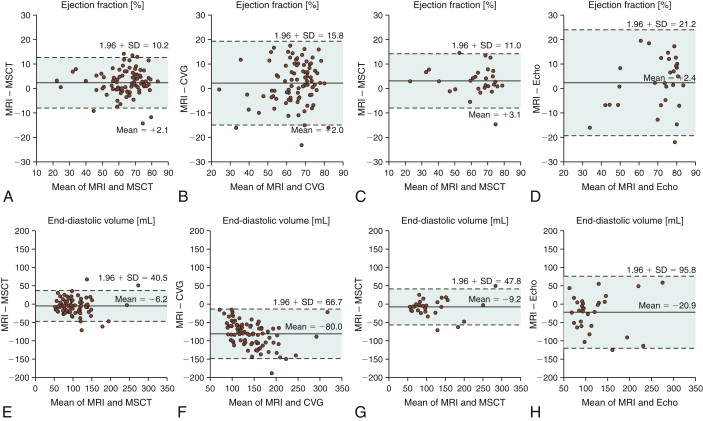
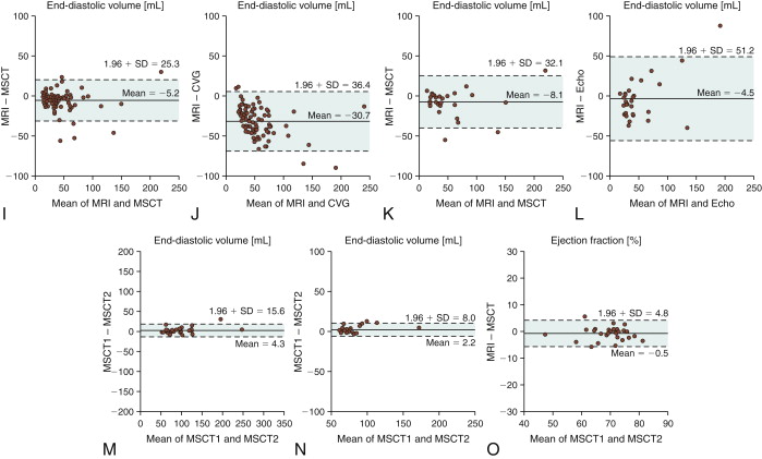
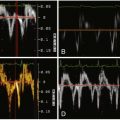
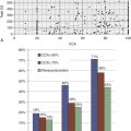
Figure 19-1
Assessment of ejection fraction: agreement between magnetic resonance imaging (MRI) and 16-slice multislice CT (MSCT) ( A ) and MRI and biplane cineventriculography (CVG) ( B ) in 88 patients. The agreement also is compared with the reference standard (MRI) for MSCT and transthoracic echocardiography (Echo) ( C and D ) in the subset of 30 patients who underwent echocardiography. The mean of the two methods compared is always plotted against the difference of the two. The solid line is the mean of the differences, whereas the dashed lines mark the limit of agreement (95% confidence intervals = 1.96 × SD) according to Bland and Altman. There were significantly larger limits of agreement for the comparison of CVG and Echo with MRI ( B and D ) than for the comparisons of MSCT with MRI ( A and C ). Agreement for assessment of end-diastolic volume between MRI and 16-slice MSCT ( E ) and MRI and CVG ( F ) in 88 patients. The agreement also is compared with the reference standard (MRI) for MSCT and Echo ( G and H ) in the subset of 30 patients according to Bland and Altman as described in Figure 20-13 . There were significantly larger limits of agreement for the comparison of CVG and Echo with MRI ( F and H ) than for the comparisons of MSCT with MRI ( E and G ), and there was also a significantly larger overestimation of the end-diastolic volume with CVG than with MSCT ( E and F ).Agreement for assessment of end-systolic volume between MRI and 16-slice MSCT ( I ) and MRI and CVG ( J ) in 88 patients. The agreement is also compared with the reference standard (MRI) for MSCT and Echo ( K and L ) in the subset of 30 patients according to Bland and Altman as described in Figure 20-13 . There were significantly larger limits of agreement for the comparison of CVG and Echo with MRI than for the comparisons of MSCT with MRI, and there was also a significantly larger overestimation of the end-systolic volume with CVG than with MSCT . Intraobserver agreement for assessment of ejection fraction ( M ), and end-systolic volume ( O ) with 16-slice MSCT in 29 patients randomly selected from the entire patient cohort. For all intraobserver analyses, the limits of agreement and the deviations from 0 were significantly smaller than for the comparison of MSCT with MRI (all P < .004) in the same 29 patients, demonstrating a low variability with MSCT.
(Reprinted with permission from Dewey M, Muller M, Eddicks S, et al. Evaluation of global and regional left ventricular function with 16-slice computed tomography, biplane cineventriculography, and two-dimensional transthoracic echocardiography: comparison with magnetic resonance imaging. J Am Coll Cardiol. 2006;48(10):2034-2044.)
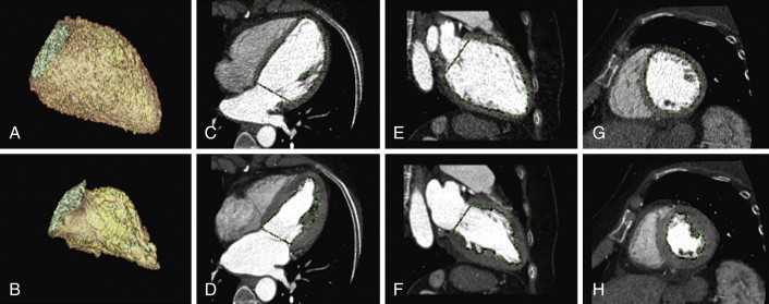
Figure 19-2
Automated cavitary delineation algorithms (unedited): diastole ( A, C, E, G ) and systole ( B, D, F, H ). Note the crisp delineation of the cavity/blood pool to the myocardium. See
- □
For CCT images of chamber quantification, see Figures 19-3 and 19-4
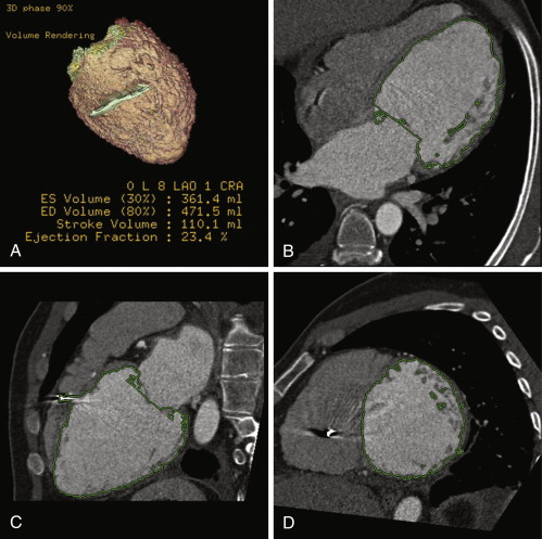
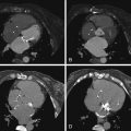
Figure 19-3
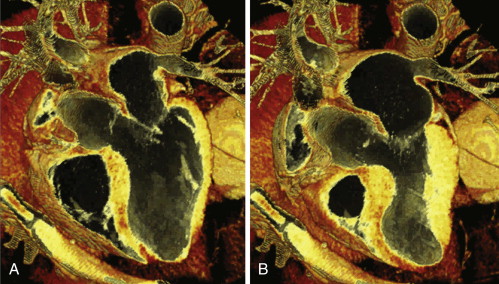
Multiple reconstructed images, helically acquired CT angiogram in patient with dilated cardiomyopathy pre-CRT therapy. A, Volume-rendered image. B through D, Automated planimetry of the LV blood volume. Because cardiac CT data sets were acquired in a four-dimensional isotropic fashion, reconstructions of various planes through the heart could easily be performed. Due to CT’s high spatial resolution and high attenuation differences between the blood pool and myocardium, automated and semiautomatic segmentation was straightforward. This patient has a severely dilated left ventricle with an end-diastolic (ED) volume of 472 mL, indexed for body surface area to 248 mL/m 2 . The left ventricular ejection fraction (LVEF) is severely decreased at 23%. ES, end-systole.
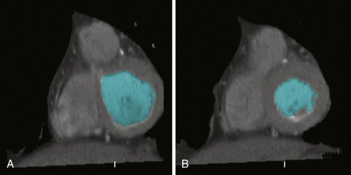
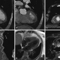
Figure 19-4
Reconstructed short-axis cine from a retrospective cardiac CT study shows an example of semi-automated left ventricular (LV) volume segmentation. Note that the mid- to distal septum demonstrates hypokinesis and corresponding hypodensity. See
- □
For plots of CCT determinations of LV mass compared with those yielded from CMR, see Figure 19-5
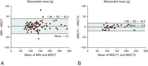
Figure 19-5
A, Agreement for assessment of myocardial mass between MRI and 16-slice multislice CT (MSCT). B, Intraobserver agreement for MSCT.
(Reprinted with permission from Dewey M, Muller M, Eddicks S, et al. Evaluation of global and regional left ventricular function with 16-slice computed tomography, biplane cineventriculography, and two-dimensional transthoracic echocardiography: comparison with magnetic resonance imaging. J Am Coll Cardiol. 2006;48(10):2034-2044.)
- □
For CCT images of LV mass calculation see Figures 19-6 and 19-7
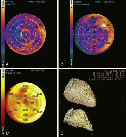
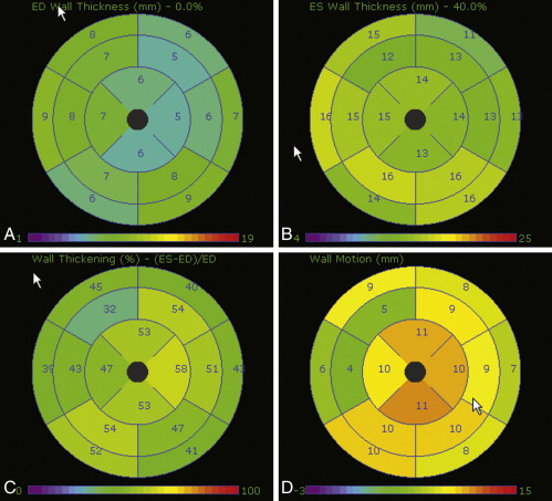
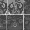
Figure 19-6
Automated calculation/plots of left ventricular wall thickness ( A ), left ventricular wall thickening ( B ), left ventricular wall motion ( C ), and left ventricular ejection fraction ( D ). 3D volume-rendered segmented reconstructions, in diastole ( D , upper image : 234 mL) and in systole ( D , lower image : 81 mL), yielding an ejection fraction of 6570. ED, end-diastolic; ES, end-systolic.
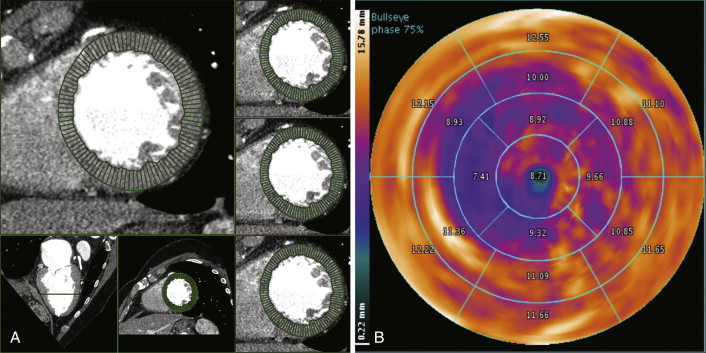
Figure 19-7
A, Automated quantification of left ventricular wall thickness. B, Segmented radial plot of wall thickness.
- □
Fine detail of the LV, such as the apical thin-point, is apparent by CT.
The principal problem is that reconstructing images from data sets at 10% intervals will not necessarily catch (true) end-systole. There tends to be more variability for CT estimations of EDV than for ESV, because trabecular topography is more variable at end-diastole.
For the validation of CCT for the assessment of LV volumes and ejection fraction, see Table 19-1 .
| AUTHOR | No. Of patients | VALIDATION | BLAND-ALTMAN ANALYSIS: BIAS (95% LIMITS OF AGREEMENT) | ||
|---|---|---|---|---|---|
| LVEDV | LVESV | LVEF (%) | |||
| Schepis et al., 2006 | 60 (known/suspected CAD) | SPECT | 34 mL (±52 mL) | 9 mL (±32 mL) | 1(±15) |
| Schlosser et al., 2007 | 21 (suspected CAD) | CMR | 19.9 mL (±20.3 mL) | 13.4 mL ±10.3 mL | 3.9 ±7.5 |
| Wu et al., 2008 | 63 (known/suspected CAD) | CMR | −0.6 mL (±29.8 mL) | 1.1 mL (±20.8 mL) | −0.2 (±8.2) |
| Nakamura et al., 2008 | 71 (known/suspected CAD) | CVG | 5.4 mL (±56.1 mL) | 7.8 mL (±29.4 mL) | −5.2 (±14.7) |
| Wu et al., 2008 | 41 (referred for CT angiography) | CMR | −1.0 mL (±43.6 mL) | 0.9 mL (±28.2 mL) | −0.1 (±12.0) |
| Abbara et al., 2008 | 22 (SPECT within 3 months) | SPECT | — | — | 0.0 (±12.5) |
| Busch et al., 2008 (dual-source CT) | 15 | CMR | 3.7 mL (±49.9 mL) | −2.6 mL (±34.mL) | 3.8 (±18.5) |
| Brodoefel et al., 2007 (dual-source CT) | 20 (suspected/known CAD) | CMR | −2.2 mL (±10 mL) | −1.4 mL (±5 mL) | 0.7 (±5) |
| Bastarrika et al., 2008 (dual-source CT) | 12 (heart transplant) | CMR | 16.6 mL (±36.5 mL) | 4.9 mL (±13.5 mL) | −0.3 (±6.2) |
| Spoeck et al., 2008 | 20 (endoscopic CABG) | CVG | — | — | 0.2 (±18.5%) |
The variability of CCT determinations of cardiac volume and systolic function is approximately half of that of real-time three-dimensional echocardiography and of CMR.
Current guidelines have classified the appropriateness of CT for evaluation of LV function post-MI or in heart failure as “uncertain” (in the context that echocardiography is technically limited). Otherwise, as a stand-alone indication, it is classified as “inappropriate,” given the availability of techniques that do not require radiation. From a clinical standpoint, in the setting of contraindications to CMR (e.g., permanent pacemakers or implantable cardioverter defibrillators) and inadequate echocardiographic imaging, cardiac CT may be particularly useful.
Assessment of wall motion is feasible. The AHA 17-segment model of the LV should be used. Cine CT is able to compile images of the heart at 10% phase intervals and to run dynamic loops ( Figs. 19-8 and 19-9 ).
The sensitivity for detection of akinesis is better than for hypokinesis, illustrating the limitations of depicting systolic function in an insufficient number of phases.
Realistically, the utility of CT-determined wall motion is generally less than that of echocardiography, CMR, or catheterization, because the temporal resolution is lower than that with these other modalities. However, assessment of wall motion is possible and the technique continues to evolve ( Table 19-2 ).
Related posts:
 Overview of the Process, Exclusions and Risks, and Preparation
 CTA Assessment of Saphenous Vein Grafts and Internal Thoracic (Mammary) Arteries
 Determination of Coronary Calcium
 Assessment of Left Ventricular Structural Abnormalities
 Cardiac and Paracardiac Masses
 Caval Anatomy: Variants and Lesions
Stay updated, free articles. Join our Telegram channel

Full access? Get Clinical Tree


