(1)
Department of Mathematics and Statistics, Villanova University, Villanova, PA, USA
Electronic supplementary material
The online version of this chapter (doi:10.1007/978-3-319-22665-1_3) contains supplementary material, which is available to authorized users.
3.1 Definition and properties
Let us begin the process of trying to recover the values of an attenuation-coefficient function f(x, y) from the values of its Radon transform  .
.
. Suppose we select some point in the plane, call it (x 0, y 0). This point lies on many different lines in the plane. In fact, for each value of  , there is exactly one real number t for which the line
  passes through (x 0, y 0). Specifically, the value
 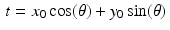 is the one that works, which is to say that, for any given values of x 0 , y 0 , and
  , the line
  passes through the point (x 0, y 0) . The proof of this fact is left as an exercise.
, there is exactly one real number t for which the line passes through (x 0, y 0). Specifically, the value is the one that works, which is to say that, for any given values of x 0 , y 0 , and , the line passes through the point (x 0, y 0) . The proof of this fact is left as an exercise.Example with R 3.1.
Figure 3.1 shows a network of back-projection lines through a selection of points in the first quadrant. This figure was created in R with the following code.
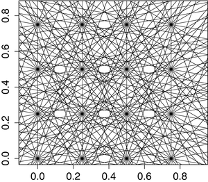
Fig. 3.1
For an array of points in the first quadrant, the figure shows the network of the back-projection lines corresponding to values of  in increments of π∕9 .
in increments of π∕9 .## plot parameterized lines for the back projection
sval1=(sqrt(2)/100)*(-100:100)#pts on each line
thetaval1=(pi/9)*(1:9-1)#9 angles
#grid of points#plot lines through these
x1=c(rep(0,4),rep(.25,4),rep(.5,4),rep(.75,4))
y1=rep(c(0,.25,.5,.75),4)
plot(c(0,.85),c(0,.85),cex=0.,type=’n’,xlab=’’,ylab=’’,
asp=1)
for (i in 1:length(x1)){
for (j in 1:Nangle){
xval=(x1[i]*cos(thetaval1[j])+y1[i]*sin(thetaval1[j]))
*cos(thetaval1[j])-sval1*sin(thetaval1[j])
yval=sval1*cos(thetaval1[j])+(x1[i]*cos(thetaval1[j])+y1[i]
*sin(thetaval1[j]))*sin(thetaval1[j])
lines(xval,yval) } }
In practice, whatever sort of matter is located at the point (x 0, y 0) in some sample affects the intensity of any X-ray beam that passes through that point. We now see that each such beam follows a line of the form  for some angle
  . In other words, the attenuation coefficient f(x 0, y 0) of whatever is located at the point (x 0, y 0) is accounted for in the value of the Radon transform
  , for each angle
  .
.
for some angle . In other words, the attenuation coefficient f(x 0, y 0) of whatever is located at the point (x 0, y 0) is accounted for in the value of the Radon transform , for each angle .The first step in recovering f(x 0, y 0) is to compute the average value of these line integrals, averaged over all lines that pass through (x 0, y 0). That is, we compute
(3.1)
Formally, this integral provides the motivation for a transform called the back projection, or the back projection transform.
Definition 3.2.
Let  be a function whose inputs are polar coordinates. The back projection of h at the point (x, y) is defined by
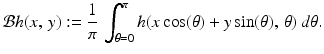
Note that the inputs for  are Cartesian coordinates while those of h are polar coordinates.
be a function whose inputs are polar coordinates. The back projection of h at the point (x, y) is defined by(3.2)
are Cartesian coordinates while those of h are polar coordinates.The proof of the following proposition is left as an exercise.
Proposition 3.3.
The back projection is a linear transformation. That is, for any two functions h 1 and h 2 and arbitrary constants c 1 and c 2 ,

for all values of x and y .
(3.3)
Example 3.4.
Back projection of  . In the context of medical imaging, the integral in (3.1) represents the back projection of the Radon transform of the attenuation-coefficient function f . That is,
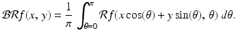
. In the context of medical imaging, the integral in (3.1) represents the back projection of the Radon transform of the attenuation-coefficient function f . That is,(3.4)
3.2 Examples
Before we rush to the assumption that (3.4) gives us f(x 0, y 0) back again, let us analyze the situation more closely. Each of the numbers  , themselves the values of integrals, really measures the total accumulation of the attenuation-coefficient function f along a particular line. Hence, the value of the Radon transform along a given line would not change if we were to replace all of the matter there by a homogeneous sample with a constant attenuation coefficient equal to the average of the actual sample’s attenuation. The integral in (3.4) now asks us to compute the average value of those averages. Thus, this gives us an “averaged out” or “smoothed out” version of f, rather than f itself. We will make this precise in Proposition 7.20 and its Corollary 7.22. For now, we’ll look at some computational examples to illustrate what’s going on.
, themselves the values of integrals, really measures the total accumulation of the attenuation-coefficient function f along a particular line. Hence, the value of the Radon transform along a given line would not change if we were to replace all of the matter there by a homogeneous sample with a constant attenuation coefficient equal to the average of the actual sample’s attenuation. The integral in (3.4) now asks us to compute the average value of those averages. Thus, this gives us an “averaged out” or “smoothed out” version of f, rather than f itself. We will make this precise in Proposition 7.20 and its Corollary 7.22. For now, we’ll look at some computational examples to illustrate what’s going on. Example 3.5.
Suppose f 1 is the attenuation-coefficient function corresponding to a disc of radius 1∕2 centered at the origin and with constant density 1. Then, for every line  through the origin, we have
 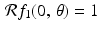 . Consequently,
 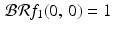 .
.
through the origin, we have . Consequently, .Now suppose that f 2 is the attenuation-coefficient function for a ring of width 1∕2 consisting of all points at distances between 1∕4 and 3∕4 from the origin and with constant density 1 in this ring. Then, again, for every line  through the origin, we get
 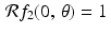 . So, again,
 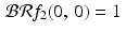 .
.
through the origin, we get . So, again, .Thus, 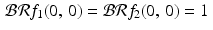 , even though f 1(0, 0) = 1 and f 2(0, 0) = 0 . This illustrates the fact that the back projection of the Radon transform of a function does not necessarily reproduce the original function.
, even though f 1(0, 0) = 1 and f 2(0, 0) = 0 . This illustrates the fact that the back projection of the Radon transform of a function does not necessarily reproduce the original function.Example 3.6.
We previously considered the function
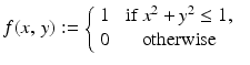 and computed that
 ,
,
 satisfy the inequality
  for an arbitrary point (x, y) . However, the maximum possible value of the expression
  is
is  , and we already know that we only care about points for which
  . Hence,
  will hold for all the points (x, y) that we care about.
Get Clinical Tree app for offline access

, satisfy the inequality for an arbitrary point (x, y) . However, the maximum possible value of the expression is , and we already know that we only care about points for which . Hence, will hold for all the points (x, y) that we care about.Now apply the back projection. Assuming, as we are, that x 2 + y 2 ≤ 1, we get
(3.5)
The three-dimensional graph of f is a circular column of height 1 with a flat top, while the graph of  , as Figure 3.2 illustrates, is a circular column with the top rounded off. This is due to the “smoothing” effect of the back projection.
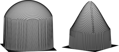
, as Figure 3.2 illustrates, is a circular column with the top rounded off. This is due to the “smoothing” effect of the back projection.Fig. 3.2
For a test function whose graph is a cylinder or a cone, the back projection of the Radon transform of the function yields a rounded-off cylinder or a rounded-off cone.
Example 3.7.
This time, let