Basic Principles of Computed Tomography Physics and Technical Considerations
Kyongtae T. Bae
Bruce R. Whiting
INTRODUCTION
Slightly more than three decades old, computed tomography (CT) continues to advance rapidly in both imaging performance and widening clinical applications. An appreciation of the potential of CT and its limitations can be obtained with an understanding of basic principles of CT operations. This chapter provides background and insight into the technical issues surrounding the application of CT, including the image formation process, various parameters affecting clinical usage, metrics to describe performance, the display of image information, and radiation dose.
Imaging with X-Rays
X-ray imaging was the first diagnostic imaging technology, invented immediately after the discovery of x-rays by Roentgen in 1895. X-rays are a form of electromagnetic energy that propagate through space and are absorbed or scattered by interactions with atoms. The attenuation of beam energy on passage through physical objects provides a noninvasive means to gather information about the amount and type of material present inside the object. In radiography, x-rays illuminate an object, resulting in a two-dimensional (2D) image that is the “shadow” of three-dimensional (3D) structures present in the beam. The projection causes a superposition of internal structures, leading to indeterminacy in the exact relationships, shapes, and relative positions of objects. Because of this indeterminacy, radiologists require extensive training and experience to interpret 3D structures from the 2D image data. Furthermore, projection radiographs have very limited ability to differentiate low-contrast differences in tissues.
Computed tomography (CT) was created in the early 1970s to overcome many of these limitations (13). By acquiring multiple x-ray views of an object and performing mathematical operations on digital data, a full 2D section of the object can be reconstructed with exquisite detail of the anatomy present (Fig. 1-1). During the years since its invention, CT technology has undergone continual improvement in performance through refinements in components and innovation in scanning techniques (19). As a result, scan times have dramatically improved, and volume coverage and resolution detail have increased.
As a curious consequence of this progress, the very large volume of image data acquired with current scanning techniques poses another challenge for interpretation: how to display very large amounts of information for the interpretation process. The magnitude and complexity of true volume imaging requires new rendering techniques to enable productive exploitation of the vast amount of information.
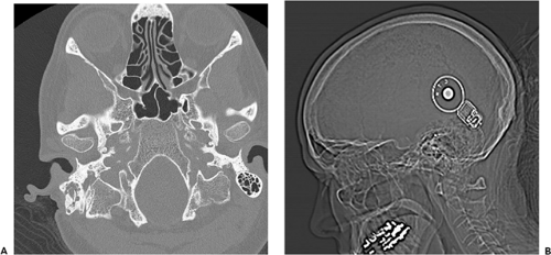 Figure 1-1 A: X-ray and B: Computed tomography of head with cochlear implant. Note the higher contrast of fine structures in the computed tomography slice, whereas superposition of structures in the x-ray confounds the three dimensional location. |
Brief History of Computed Tomography
Since its introduction in the mid-1970s, CT scanner technology has undergone a continual improvement in performance, including increases in acquisition speed, amount of information in individual slices, and volume of coverage. A graph (Fig. 1-2) of these parameters versus time looks similar to Moore’s Law for computer price-performance, which observes that computer metrics (clock speed, cost of random access memory or magnetic storage, etc.) double every 18 months. In the case of CT technology, the doubling period is approximately 32 months, still an impressive rate. For example, scan time per slice has decreased from 300 seconds in 1972 to 0.005 seconds in 2005. Factors contributing to this remarkable advance include improvements in electronics hardware and development of innovative mechanical scanning configurations.
Historically, the early scanner configurations were characterized as successive generations of scanner geometry (Fig. 1-3). By 1990 rotating fan beam systems, utilizing slip-ring technology to allow continuous rotation of x-ray tube and detector, had reduced acquisition time to about 1 second, with reconstruction computations requiring several seconds per slice. Nevertheless, the time required to scan a patient volume of interest often was longer than a single breath-hold, and scan range was limited by x-ray tube heat load to 10 to 30 cm. By translating the patient table continuously through the rotating gantry, termed helical or spiral scanning, volume coverage and scan speed were further increased, with fundamental rate limitations being x-ray
tube output and mechanical rotation rate. Image reconstruction techniques were developed to interpolate 2D planes from the 3D datasets that were acquired in helical mode. In the late 1990s, the obstacles encountered by early helical scanners were overcome by multidetector row technology, using multiple sets of detector rows to utilize more of the x-ray tube output and acquire measurements at multiple section levels in parallel. Reconstruction under these conditions is inherently 3D, so more complex algorithms must be used. Benefiting from substantial improvements in computing power, the rapid increases in CT performance appear to be sustainable into the new century, with development of flat panel detectors, faster electronics, and cone-beam geometry reconstruction algorithms.
tube output and mechanical rotation rate. Image reconstruction techniques were developed to interpolate 2D planes from the 3D datasets that were acquired in helical mode. In the late 1990s, the obstacles encountered by early helical scanners were overcome by multidetector row technology, using multiple sets of detector rows to utilize more of the x-ray tube output and acquire measurements at multiple section levels in parallel. Reconstruction under these conditions is inherently 3D, so more complex algorithms must be used. Benefiting from substantial improvements in computing power, the rapid increases in CT performance appear to be sustainable into the new century, with development of flat panel detectors, faster electronics, and cone-beam geometry reconstruction algorithms.
 Figure 1-2 Evolution of computed tomography scanner performance: plot of acquisition performance versus time, for computed tomography scanners. The slope implies a doubling of performance approximately every 2 years. (Data from Siemens Medical Systems, http://www.medical.siemens.com, “CT History and Technology.”). |
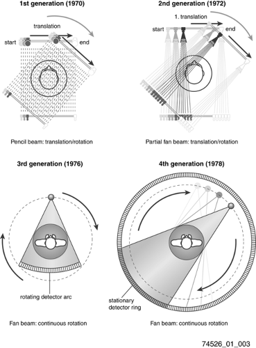 Figure 1-3 Definition of the different generations of scan geometries. |
To understand best how to utilize CT technology clinically and appreciate new product capabilities, knowledge of fundamental CT imaging principles is necessary. The basic principles of CT involve physical mechanisms that are shared with x-ray imaging, plus mathematical techniques that exceed the human visual perception of 2D images. A common technical description can be used to describe both the image formation process and the image visualization task. These will now be examined in detail.
COMPUTED TOMOGRAPHY ACQUISITION SYSTEM COMPONENTS
Generation of X-Rays
For medical imaging, x-rays are generated by an x-ray tube. In this device, a metal filament is heated (much like a light bulb) until energetic electrons escape from the cathode
surface into a vacuum. These electrons are then accelerated by an electric field, acquiring kinetic energy while being attracted to a positive anode target. The total amount of energy acquired by the electron in the accelerating electric field is equal to the product of the potential (peak kilovoltage, kVp) times the unit of electrical charge, possessing units of electron volts (kilo electron volts, keV). The amount of charge generated by the x-ray tube per unit time has units of electrical current (milliamperes, mA), and the product of voltage and current is the amount of power (watts) delivered by the tube. Electrostatic and/or magnetic fields are used to focus the electron beam into a small area of the anode target. Typically, this focal spot has dimensions of about 1 mm. When the electrons collide with the target, most of their energy is dissipated into heat but a small fraction (<1%) is converted into several forms of electromagnetic radiation. A typical spectrum of the distribution of energy emitted by the x-ray tube is shown in Figure 1-4. Characteristically, there is a linearly decreasing portion caused by bremsstrahlung, the deceleration of the electrons in the target. According to Maxwell’s equations, any charge undergoing acceleration will radiate electromagnetic energy. As beam electrons pass through target atoms, they interact and are accelerated. The maximum amount of energy that can be transferred is equal to e × kVp, and lesser amounts of energy appear randomly depending on the details of electron collisions. The sharp peaks in the spectrum occur when the beam electrons deposit energy by exciting atomic electrons in the target. Electron shell transfers arise in atoms, with characteristic radiation at well-defined (K-edge) energy peaks.
surface into a vacuum. These electrons are then accelerated by an electric field, acquiring kinetic energy while being attracted to a positive anode target. The total amount of energy acquired by the electron in the accelerating electric field is equal to the product of the potential (peak kilovoltage, kVp) times the unit of electrical charge, possessing units of electron volts (kilo electron volts, keV). The amount of charge generated by the x-ray tube per unit time has units of electrical current (milliamperes, mA), and the product of voltage and current is the amount of power (watts) delivered by the tube. Electrostatic and/or magnetic fields are used to focus the electron beam into a small area of the anode target. Typically, this focal spot has dimensions of about 1 mm. When the electrons collide with the target, most of their energy is dissipated into heat but a small fraction (<1%) is converted into several forms of electromagnetic radiation. A typical spectrum of the distribution of energy emitted by the x-ray tube is shown in Figure 1-4. Characteristically, there is a linearly decreasing portion caused by bremsstrahlung, the deceleration of the electrons in the target. According to Maxwell’s equations, any charge undergoing acceleration will radiate electromagnetic energy. As beam electrons pass through target atoms, they interact and are accelerated. The maximum amount of energy that can be transferred is equal to e × kVp, and lesser amounts of energy appear randomly depending on the details of electron collisions. The sharp peaks in the spectrum occur when the beam electrons deposit energy by exciting atomic electrons in the target. Electron shell transfers arise in atoms, with characteristic radiation at well-defined (K-edge) energy peaks.
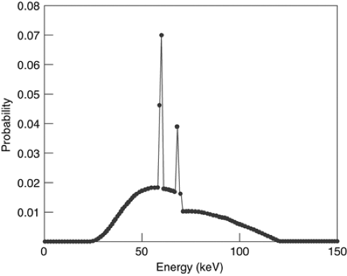 Figure 1-4 Typical x-ray spectrum for tungsten target with 120 kVp. Low-energy photons, which do not pass through the patient to contribute to final image, have been filtered out. |
The spectrum generated in an x-ray tube contains many low energy photons. The power in the beam associated with a particular energy range is fairly constant, because the number of quanta decreases linearly as a function of energy, while the energy of an individual quantum increases linearly. Because the lowest energy quanta are effectively attenuated in the patient, they contribute very little to the measured signal while exposing the patient to radiation dose. Therefore, the beam is filtered by placing material around the x-ray tube to reduce much of the low energy quanta while passing high energy quanta, leading to an optimal image quality/dose tradeoff.
The x-rays from the target are spread over a wide solid angle (essentially a hemisphere). To minimize radiation dose and generation of background scatter, the x-ray beam is collimated by an aperture into a thin fan beam. For CT scanners, the beam is typically a few millimeters thick in the patient, subtending a fan of about 45 degrees. Additionally, because human anatomy typically has a round cross-section that is thicker in the middle than in the periphery, more x-ray flux reaches detectors in the center than on the edges. This means that patients receive more dose than is necessary on the periphery of their anatomy. To compensate for this effect, a bowtie-shape filter is placed in the beam, which is tapered such that its center is thinner than its edges, to equalize the flux reaching the detectors and minimize patient dose.
The inefficiency in conversion of electron current into x-rays has been a significant practical limitation in the operation of x-ray imaging equipment. The tube is quickly heated to high temperatures, which must be limited to avoid damage. Anode targets have been designed to rotate on bearings, spreading out the area that is heated by the beam. Heat sinks are used to remove heat from the system by convection or water-assisted cooling.
In typical clinical operation, an x-ray tube delivers on the order of 2 × 10¹¹ x-rays per second to the patient, providing a high signal-to-noise ratio for measurements.
Detection of X-Rays
Detection of x-rays is accomplished by the use of special materials that convert the high energies (tens of keV) of the x-ray quantum into lower energy forms, such as optical photons or electron-hole pairs, which have energies of a few electron volts. In this down-conversion, many secondary quanta are generated, typically thousands per primary quanta. The detector materials, such as phosphors, scintillating ceramics, or pressurized xenon gas, ultimately produce an electrical current or voltage. Electronic amplifiers condition this signal, and an analog-to-digital converter converts it into a digital number. The range of signals produced in tomography is large, varying from a scan of air (no attenuation, or 100% transmission) to that of a large patient with metal implants (possible attenuation of 0.0006%), a factor of almost 105. Furthermore, even at the lowest signal levels, the analog-to-digital converter must be able to detect modulations of a few percent. Thus the overall range approaches a factor of one million, specifying the equivalent of a 20-bit analog-to-digital converter.
Gantry Electromechanics
To obtain required measurements at different angles, all the electrical components must be rotated around the patient. In modern scanners, this puts tremendous requirements on mechanical precision and stability. The gantry can weigh 400 to 1,000 kg, span a diameter of 1.5 m, and rotate 3 revolutions per second. While rotating, it may not wobble more that 0.05 mm.
Originally, the gantry was connected by cables to the outside environment and had to change rotation direction at the end of each revolution. A major breakthrough in scanning operation occurred with the invention of slip-ring technology, which used brush contacts to provide continuous electrical power and electronic communication, allowing continuous rotation.
Helical/Spiral Scanning
One of the primary goals of CT manufacturers has been to provide faster scan times and larger scan coverage. With the advent of slip-ring technology and continuous gantry rotation, the main limitation to scanning speed was the stepping of the patient bed to position sequential slices. In the late 1980s continuous motion of the patient table was introduced, which allowed faster scan times but required different data handling for image reconstruction (Fig. 1-5). Previously the theory of CT reconstruction was based on having a complete set of gantry measurements for each slice reconstructed. However, in helical scans the gantry is at continuously different table positions throughout each rotation. A good mathematical approximation for each gantry position is to interpolate a reconstruction plane from corresponding neighboring gantry positions. This approach provided adequate image quality, and in fact had the added benefit that slices could be reconstructed retrospectively for arbitrary table positions, instead of being limited to fixed table increments. Furthermore, analysis revealed that on average the spatial resolution was better with helical scans rather than sequential scans. A drawback was that the interpolation process could create stair-step artifacts on the boundaries of extended high-contrast objects.
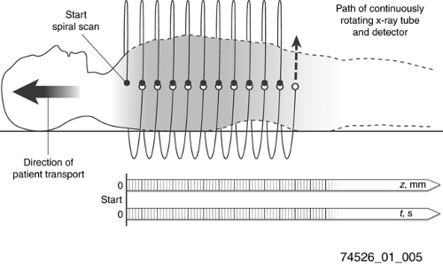 Figure 1-5 Helical or spiral scanning involves translating the patient longitudinally through the rotating gantry. |
Detector Configuration
By the mid-1990s, helical scans had become limited in speed because of the mechanical forces associated with subsecond gantry rotation times and the output requirements of x-ray tubes to supply enough flux for adequate signal to noise ratio. The next improvement in performance resulted from acquiring measurements at multiple body levels in parallel, using more than one row of detectors at the same time. This advance allowed an increase in speed of volume acquisition proportional to the number of rows of detectors. In this approach, the x-ray tube produces a broad beam of x-rays, rather than one that is collimated to a narrow slice; by widening the collimation to illuminate multiple rows of detectors, more measurements are acquired from the same tube output. Initially, two- or four-row multidetector row CT (MDCT) scanners were introduced, but the number of detector rows has grown steadily, with 64-detector row devices now enabling very large volume coverage. Because of the increased longitudinal width of the x-ray beam with MDCT, image data measurements no longer correspond to rays orthogonal to the scan axis; thus new reconstruction algorithms are required to maintain image quality and prevent distortions.
In single-detector row CT (SDCT), each individual detector row functions as a single unit and provides projection data for a single section per rotation. In SDCT, different section widths are obtained by means of adjusting prepatient collimation of the x-ray beam (Fig. 1-6). In MDCT, the detectors are further divided along the z-axis, allowing simultaneous acquisition of multiple sections per rotation. Thus MDCT provides larger and faster z-axis coverage per rotation with thinner section widths.
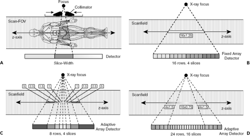 Figure 1-6 Multidetector computed tomography configurations. A: Illustration shows prepatient collimation of the x-ray beam to obtain different collimated section widths with a single-detector row computed tomography detector. FOV = field of view. Illustrations show examples of (B) fixed-array and (C, D) adaptive-array detectors used in commercially available four-section and 16-section computed tomography systems. |
When four-channel MDCT scanners were introduced in the late 1990s, three different detector configurations were used by the CT manufacturers: (A) 16 detector rows with a uniform thickness, termed uniform array (General Electric); (B) eight detector rows of variable thicknesses, thinner rows centrally and wider rows peripherally, termed adaptive array [Siemens and Philips]; and (C) 34 detector rows with two fixed thicknesses, four thinner rows centrally and 30 thicker rows peripherally, termed hybrid array (Toshiba). Note that four-channel MDCT systems contain detectors that are divided into eight to 34 rows along the z-axis. Nevertheless, the number of sections acquired at each rotation is restricted to four because these systems contain only four data channels. When a scan with a narrow collimation is desired, four individual central detector rows are used for the data measurement, with a narrowly collimated x-ray beam directed over these central detector rows (e.g., 4 × 1 mm). To generate scans with larger section widths, a broadly collimated x-ray beam is used, and outputs from two or more adjacent detector rows are electronically combined into a single thicker detector row for each of the four data channels. For example, two 1-mm detector rows can be grouped to function as a single detector row for 2-mm collimation (4 × 2 mm), three 1-mm detector rows for 3-mm collimation (4 × 3 mm), and so on.
For 16-channel MDCT, all of the CT manufacturers adopted a hybrid array design, in which the thickness of the detector rows is slightly less than 1 mm for the central rowsand slightly more than 1 mm for the peripheral rows. However, the length of the z-axis coverage and the number of detector rows varies widely among the CT manufacturers.
For 64-channel MDCT, the CT manufacturers have again used a common detector row design, this time a uniform array in which all the detector rows have a uniform thickness. However, as in 16-channel MDCT, the total number of detector rows and the z-axis coverage are highly variable among the CT manufacturers.
COMPUTED TOMOGRAPHY IMAGE FORMATION
X-Ray Signals
X-ray imaging consists of the generation of x-rays, transmission of those x-rays through material objects, and the detection of the beam energy that exits the object. The attenuation of x-rays within an object is governed by interactions on the atomic scale, in which each molecule in the object has some cross section for interacting with each x-ray. Because of this interaction, the x-ray flux decreases on
average by a certain percentage for each unit distance traveled through the object. Thus, if a 60 keV x-ray travels through 1 mm of water, on average it will survive 97.4% of the time. For 2 mm of water, the survival probabilities multiply for a 95% rate. The transmission probability is thus an exponentially decreasing function of the total amount and type of material present, represented by Lambert-Beer equation:
average by a certain percentage for each unit distance traveled through the object. Thus, if a 60 keV x-ray travels through 1 mm of water, on average it will survive 97.4% of the time. For 2 mm of water, the survival probabilities multiply for a 95% rate. The transmission probability is thus an exponentially decreasing function of the total amount and type of material present, represented by Lambert-Beer equation:
where S is the number of surviving signal quanta, I is the number of incident quanta, the subscript i indicates different materials that are compose the sample, μi is the linear attenuation coefficient for each material and μi is the amount (thickness) of that material present.
In projection x-ray imaging, the image consists of the relative changes in the signal S across a viewing area. For a 70-kg person, with an abdomen roughly equivalent to 20-cm thickness of water, the survival probability for a single quantum would be about 2%. The presence of an additional 2 mm of abnormal structure would change this survival probability to 1.98% (only a 1% difference). Given this small change in the midst of many overlapping body structures, it is clear that projection radiography is limited in its ability to demonstrate anatomic details. In CT imaging, measurements of S are made from multiple projections, and from these measurements μi is computed for direct display. This technique results in much higher relative contrast between adjacent structures. For example, a 2-mm calcified nodule may have a 200% difference in attenuation coefficient compared with surrounding tissue, and hence be much more conspicuous than on a projection radiograph (see Fig. 1-1).
For the viewing of images, projection x-rays are presented as a brightness that is proportional to the changes of the transmitted signal S in Eq. 1. In CT, the image attenuation map is presented in units that are relative to the attenuation coefficient of water, expressed as Hounsfield units (HU).
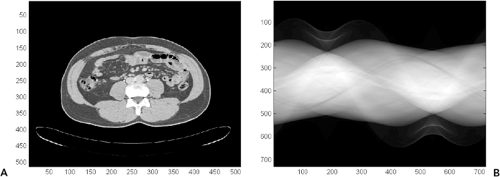 Figure 1-7 An abdominal slice and its sinogram. |
Image Reconstruction From Two-Dimensional Projection Data
The basics of CT image generation can be illustrated by the reconstruction of a 2D image section from projection measurements. An x-ray source and a set of detectors rotate around the patient, making measurements of the transmission of x-rays through the body. Each measured value is the result of all the attenuating portions in the patient along a line from the x-ray source to the detector making the measurement. Hence, a uniform circular disk will have highest attenuation in its center, with a circular profile. The collection of line measurements from different view angles during one revolution of the gantry provides raw projection data prior to reconstructing images. The raw projection data result in a sinogram (Fig. 1-7). The sinogram can be displayed as an image, with the y-axis (rows) representing the measurements of each detector and the x-axis (columns) representing detector measurements at one gantry position. The sinogram image has an intriguing pattern, but is difficult to interpret because of the overlapping shapes. Thus, a method is needed to derive and compute the original image attenuation.
One method, albeit impractical, for determining the source image involves treating the sinogram and image as a linear algebra problem. Each measurement is an equation summing all the image pixels along a ray to the detector; the set of all equations can then be solved for the image pixel unknowns. The size of this problem is dauntingly large because there are 512 × 512 (i.e., more than one quarter million) variables involved with 768 × 1,400 (i.e., more than one million) measurements, requiring matrix operations that overwhelm even modern computers. Other mathematical methods, such as iterative techniques or maximum likelihood optimization, can be used to solve for images, but they also are too computationally intensive for routine clinical usage.
The mathematical process that made CT reconstruction practical is called filtered back projection. It can be shown theoretically (5) that if the projection measurements have certain properties (they all lie in one plane, they consist of
equally spaced gantry steps covering at least one half revolution, and the detectors are equidistant and cover the whole object to be reconstructed), then the attenuation (image) at any point within the scanner field of view can be calculated by summing a certain weighted combination of the measurements. This weighted summation process is called a kernel (see the section titled Reconstruction Kernel later in this chapter for detail). The measurement of the detector directly intercepting the pixel is added and measurements from neighboring detectors are subtracted. Different kernels can be designed to provide sharp, crisp images or to smooth out noise, depending on the clinical application. This process, which was universally adopted by CT manufacturers in the early years of CT, can be performed very efficiently by computers or special hardware modules, either directly or with Fast Fourier Transform techniques.
equally spaced gantry steps covering at least one half revolution, and the detectors are equidistant and cover the whole object to be reconstructed), then the attenuation (image) at any point within the scanner field of view can be calculated by summing a certain weighted combination of the measurements. This weighted summation process is called a kernel (see the section titled Reconstruction Kernel later in this chapter for detail). The measurement of the detector directly intercepting the pixel is added and measurements from neighboring detectors are subtracted. Different kernels can be designed to provide sharp, crisp images or to smooth out noise, depending on the clinical application. This process, which was universally adopted by CT manufacturers in the early years of CT, can be performed very efficiently by computers or special hardware modules, either directly or with Fast Fourier Transform techniques.
Image Reconstruction from Three-Dimensional Projection Data
The filtered back projection process requires that the image data be confined to a single plane. With helical CT, 3D volumes rather than single sections of data are acquired, necessitating the development of new reconstruction algorithms.
Single-Detector Row Spiral Computed Tomography: Linear Interpolation
In spiral scanning, the patient table moves continuously, so at any given longitudinal or z-location there are only a few (or no) exactly corresponding gantry measurements that are aligned in the same plane for 2D filtered back projection. The higher the pitch (i.e., the faster the CT table travels relative to the detector collimation), the more the gantry measurements separate and deviate from the plane. To provide a complete set of measurements for filtered back projection, missing gantry measurements are estimated by taking the average of the closest (in the z-axis) measurements that are collected.
Two versions of this method are employed. The first is called 360LI and takes averages of measurements separated by one rotation. In this approach, to generate projection data for a target image plane, two gantry measurements on either side of the image plane that are positioned closest to the image plane and are 360 degrees apart (i.e., are measured in subsequent rotations) are linearly interpolated for each projection angle. The 360LI technique has the disadvantage that the travel in one revolution may be large, and if structures change significantly over this distance blurring or partial volume averaging will result.
The second method, called 180LI, takes advantage of the symmetry between x-ray source and detector across the gantry, i.e., the measured ray is nominally the same when the source-detector positions are one half rotation (180 degrees) apart. The 180LI technique makes use of the fact that for each measurement ray, an interpolation partner is already available after approximately one half a rotation, when the x-ray tube and detector have switched positions. This virtual, geometrically derived ray is called a complementary ray. The 180LI technique involves smaller z-distances and hence suffers less blurring. (The same trick can be used in cardiac imaging, to shorten the time window for an image snapshot and minimize temporal blur.)
Multidetector Row Spiral Computed Tomography: Z-Interpolation or Z-Filtering
The first multidetector row scanners had two or four detector rows, and the data measurements could be treated as a simple parallel stack of independent detector rows. In this case, the 360LI and 180LI used in SDCT spiral reconstruction approaches can be directly extended to spiral MDCT. One could then create planes of measurements by linear interpolation (either 360LI or 180LI) from the closest row measurements to the target plane, a technique known as advanced single-slice rebinning (29). The interpolation calculation can be performed very rapidly and is essentially similar to single-row scanning. In the 360LI interpolation approach, the interpolation can be performed using rays measured at the same projection angle by different detector rows or in consecutive rotations of the scanner 360 degrees apart. In the 180LI reconstruction approach, both direct and complementary rays can be used for spiral interpolation. CT scanner manufacturers proposed different mathematical approaches for weighting and interpolating neighboring rays for the target image plane, such as z-interpolation or z-filtering (3,22,25).
Broad Beam Multidetector or Flat-Panel Computed Tomography: Cone Beam Reconstruction
With increases in the number of detector rows beyond four, it becomes necessary to account for the cone-beam angle between detector rows (8). Some manufacturers use variations and extensions of nutating-section algorithms for image reconstruction (4,16,21,31). These algorithms split the 3D reconstruction task into a series of conventional 2D reconstructions on tilted intermediate image planes, thereby benefiting from established and very fast 2D reconstruction techniques. Examples are adaptive multiplanar reconstruction (Siemens) (7) and the weighted hyperplane reconstruction (GE Medical Systems) (12) techniques. Other manufacturers (Toshiba, Philips) have extended to multisection scanning the Feldkamp algorithm (6,9), an approximate 3D convolution back-projection reconstruction that was originally introduced for sequential scanning. With this approach, accounting for their cone-beam geometry, the measurement rays are back projected into a 3D volume along the lines of measurement. Three-dimensional back projection is, however, computationally demanding and requires dedicated hardware to achieve acceptable image-reconstruction times. The development of methods to account for the cone-beam geometry of the measurement x-rays currently is an active area of research.
IMAGING METRICS
Although image quality is the ultimate measure of an imaging system, it is difficult to define and quantify image quality. In clinical settings, image quality is frequently determined qualitatively and subjectively. Communication theory specifies the fundamental parameters of information transfer as signal, resolution, distortion, and noise to characterize system performance. Several quantitative and objective parameters are commonly used to describe image quality: spatial resolution, contrast resolution, temporal resolution, noise, and artifacts. These parameters are affected by CT scanner apparatus and scan variables and are often used to assess the performance of a CT scanner.
Signal
An image represents a map of some physical quantity, either directly measured or derived from measurements. The image signal can be continuous, as in a screen-film x-ray or 35-mm photograph, or they can be discrete, such as a medical image on a computer monitor. In the CT acquisition process, the quantity measured is the attenuation of the x-ray beam (just like a projection x-ray), with a continuous physical electrical signal representing x-ray energy flux, converted to a discrete digital value. From a set of these measurements, a digital image is calculated to represent the attenuation coefficient of the material in the object. The map is a collection of pixels (picture elements), typically a square array of 512 pixels on a side. When multiple slices are collected into volume data sets, the 3D map becomes a collection of voxels (volume elements). In computer terms, the original measurements may consist of 16-bit data (allowing a range of values spanning a factor of 64,000), whereas the reconstructed images typically are 8- or 12-bit data (a range up to 4,095). It is assumed that the signal is linear with the physical properties of the displayed object. For example, if the density of the contrast medium in a voxel doubles, the pixel value will increase by a factor of two.
The information in the image signal consists of patterns of change in the image. The magnitude of such change is characterized by contrast, the variation of local values from the surrounding values. In discrete, digital systems, the bit depth of the data determines the smallest change recordable, typically 0.02% step (12 bits) in the digital data or 0.4% step (8 bits) for a displayed image.
In the image display process, signal relates to the intensity of light patterns that a human observer views. The dynamic range of light signal may be a factor of 500 to -1,000 from light to dark. Signals can be transformed into different representations, e.g., a CT attenuation image file gets mapped to a light intensity signal for viewing on a monitor, with brightness and contrast adjustments to emphasize different areas of interest.
Resolution
The term resolution characterizes the ability of an imaging system to detect changes in a signal; the term arises in several different contexts in image operations (e.g., spatial or temporal resolution). The ability of an imaging system to record changes between different points in space depends on two factors: system aperture and (for discrete systems) sampling rate. A system aperture can take different forms: in a display system, it may be the size of the spot of light to form the image; in a CT scanner, it could be the size of the detector cell that measures the x-ray flux. The aperture is considered piece-wise constant within itself, so changes can only be recorded over a size commensurate with its dimensions. Spatial resolution is characterized by a point spread function, which is the signal footprint of an infinitesimal size (point) input, and is expressed as length (such as full-width at half maximum value of the point spread function). Equivalently, the resolution can be reported in the frequency domain by describing a modulation transfer function (MTF), which characterizes how signals of different spatial frequencies (size) are attenuated by the measuring system.
In discrete systems, an additional factor affecting resolution is the sampling rate at which signals are transferred. For example, a moving light beam 1 mm in diameter might be modulated every 0.5 mm. Elegant mathematical analyses exist for describing the effect of sampling rate on signal information. One often used result is the Nyquist criterion, which states that at least two samples are required over the distance of the system aperture to prevent distortion of signal information. Such analysis is used extensively in designing medical imaging systems.
Spatial (High-contrast) Resolution
Spatial resolution measures the capability of an imaging system to resolve closely placed objects or to display fine details. The spatial resolution of CT is described in two dimensions, xy-image (in-plane) resolution and z-direction (longitudinal) resolution. In-plane and longitudinal resolution depend on different factors. Traditionally the in-plane spatial resolution has been far better than the longitudinal or cross-plane spatial resolution, but the longitudinal resolution has been significantly improved with MDCT and approaches that of the in-plane resolution.
In-Plane Spatial Resolution
In-plane spatial resolution is usually expressed in line pairs per millimeter, typically 0.5 to 2 lp/mm for CT. It is often measured directly by imaging and visualizing high-contrast objects of increasingly smaller sizes or increasing spatial frequencies (Fig. 1-8). However, the evaluation process involved in this approach may be subjective. More objective, quantitative methods are based on calculation of MTF, which is defined as the ratio of the output modulation to the input modulation, measuring the response of
an imaging system to different frequencies. The MTF is most commonly obtained by taking a Fourier transformation of the point spread function that is measured by scanning the cross-section of a thin wire phantom. It is expressed by a plot of the fraction of subject contrast in the image versus spatial frequency. Spatial resolution is then specified at the frequency for a given percent value of the MTF (Fig. 1-9).
an imaging system to different frequencies. The MTF is most commonly obtained by taking a Fourier transformation of the point spread function that is measured by scanning the cross-section of a thin wire phantom. It is expressed by a plot of the fraction of subject contrast in the image versus spatial frequency. Spatial resolution is then specified at the frequency for a given percent value of the MTF (Fig. 1-9).
Related posts:


Stay updated, free articles. Join our Telegram channel

Full access? Get Clinical Tree


