Introduction
The heart is characterized by a complex electromechanical activity essential for the sustenance of body function. Cardiac disease is the leading cause of morbidity and mortality in the industrialized world,1 imposing a major burden on health care systems. Current therapies rely, to a large extent, on implantable devices, administration of drugs, or the ablation of tissue. Although these therapies may improve a patient’s condition significantly, they are palliative rather than curative, and undesired adverse effects of varying degrees of severity are quite common.2-5 In the quest of devising novel, safer, and more effective therapies to reduce medical costs and treatment duration, developing a comprehensive understanding of cardiac structure and function in health and disease is the strategy most likely to succeed and, thus, is a central focus of basic and clinical heart research. Traditionally, experimental work in conjunction with clinical studies was the dominant, if not exclusive, approach for inquiries into physiological function. Today, in the postgenomic era, a wider portfolio of techniques is employed, with computational modeling being another accepted approach, either as a complement to experimental work or as a stand-alone tool for exploratory testing of hypotheses. The need for computational modeling is mainly driven by the difficulty in dealing with the vast amount of available data, obtained from various subsystems of the heart, at different hierarchical levels of organization from different species, and with the complexity involved in the dynamics of interactions between subsystems within and across levels of organization. Computational modeling plays a pivotal, if not indispensable, role in harnessing these data for further advancing our mechanistic understanding of cardiac function.
Over the past decade, impressive advances in experimental technology have generated a wealth of information across all levels of biological organization for various species, including humans, ranging from the genetic scale of the cardiac system up to the entire organ. However, attempts to translate these large quantities of experimental data into safer and more effective therapies to the benefit of patients have largely proved to be elusive. In no small part, this results from the complexity of biological systems under study. They invariably comprise multiple subsystems, interacting with each other within and across levels of organization. Although biological systems can be dissected into many subcomponents, there is now a clear recognition that the interaction within and across levels of organization may produce emergent properties that simply cannot be predicted from “reductionist” analysis. Because these emerging properties are often not intuitive and not predictable from analyzing the subsystems in isolation, detailed understanding of individual subsystems may provide little mechanistic insight into functions at the organ level.6 Moreover, due to the highly complex nonlinear relationship between a rapidly increasing amount of disparate experimental data on an increasingly larger number of biological subsystems involved, any attempts to gain new mechanistic insights at the level of a system by deriving a qualitative understanding of all the simultaneous interactions within and between subsystems simply by reasoning are futile. Due to the complexity of the system, conclusions may even be misleading and, most likely, will not withstand thorough quantitative scrutiny. Integrative research approaches are required to address these issues, and computational modeling is a key technology to achieve such integration.
Furthermore, computer modeling can aid in overcoming the numerous limitations of current experimental techniques by complementing in vivo or in vitro experiments with matching in silico* models. The most common experimental limitations include the following. (1) Current experimental techniques cannot resolve, with sufficient accuracy, electrical events confined to the depth of the myocardial walls, which limits observations to the surfaces of the heart. (2) Selectively changing a single parameter in a well-controlled manner without affecting any other important parameters of cardiac function is difficult because the technology required is not available or because sufficiently selective substances have not been developed yet. (3) Certain experimental techniques require modification of the substrate or the knock-out of other physiological functions. For instance, to optically map cardiac electrical activity, first, photometric dyes are required, which modify membrane physiology and are known to be cytotoxic, and second, electromechanical uncouplers are administered to suppress mechanical contraction, further modulating physiological function. Caution is advised when interpreting such data because potentially important regulatory mechanisms are excluded.7 (4) Experimental studies are mainly performed in animals, but species differences in the distribution and kinetics of ion channels are significant. As a result, drugs, for instance, may have significantly different effects in humans than in other species. (5) Due to the invasive nature, most advanced experimental methods are limited to animal studies and cannot be applied clinically to humans. Hence, available data from human studies are very limited, and available animal models do not adequately reflect the evolution of cardiovascular diseases in people.
*In silico refers to performed on a computer via a computer simulation.
Biophysically detailed cell modeling was introduced as early as 1952 in neuroscience, through the seminal modeling work of Hodgkin and Huxley on the squid giant axon.8 Pioneered by Noble in the 1960s,9 first models of cardiac cellular activity were proposed, but the first computer models for studying bioelectric activity at the tissue level did not emerge until the 1980s.10 By today’s standards, the level of detail in early modeling work was very limited. Computational performance was poor, efficient numerical techniques had not been fully developed, and descriptions of cellular dynamics were lacking many details. To keep simulations tractable, the cardiac geometry was approximated by geometrically very simple structures such as one-dimensional (1D) strands, two-dimensional (2D) sheets,11,12 and three-dimensional (3D) slabs.13 Although geometrically simple models continue to be used, due to their main advantage of simplicity, which facilitates the dissection of mechanisms, it became quickly recognized, maybe unsurprisingly, that observations made at the organ level cannot be reproduced without accounting for organ anatomy. The combined effects of structural complexity and the various functional heterogeneities in a realistic heart led to complex behavior that is hard to predict or investigate with overly simplified models. Besides computational restrictions, simple geometries were also popular because electric circuitry analogs could be used to represent the tissue as a lattice of interconnected resistors or a set of transversely interconnected core-conductor models.11 Thus, well-established techniques for electric circuit analysis could be applied, and simple discretization schemes based on the finite difference method became a standard due to their ease of implementation. With the advent of continuum formulations,14 derived by homogenization of discrete tissue components,15 and the adoption of more advanced spatial discretization techniques such as refined variants of the finite difference method,16,17 the finite element method,18,19 and the finite volume method,20,21 the stage was set for anatomically realistic models of the heart. During the past few years, anatomically realistic computer simulations of electrical activity in ventricular slices,22-24 whole ventricles,25-28 and atria29-31 have become accessible. Such models are considered as state-of-the-art; nonetheless, many simplifications persist:
- The geometry of the organ is represented in a stylized fashion (“one heart geometry fits all” approach)25,26; only parts of the heart are modeled, such as slices across the ventricles.22
- The computational mesh discretization is coarser than the size of the single cell (100 μm) to diminish the degrees of freedom in the model. This approach leads to (1) underrepresentation of (to the degree of fully ignoring) the finer details of the cardiac anatomy, such as endocardial trabeculations or papillary muscles and (2) the necessity to adjust, in an ad-hoc manner, the tissue conductivity tensors in order to avoid artificial scaling of the wavelength, thus compensating for the dependence of conduction velocities on grid granularity. That is, as the grid is coarsened with all other model parameters remaining unchanged, conduction velocity becomes reduced, and thus, the wavelength is diminished, with conduction block occurring above a certain spatial discretization limit.
- The myocardial mass is treated as a homogeneous continuum, without representing intramyocardial discontinuities such as vascularization, cleavage planes, or patches of fat or collagen.
- The specialized cardiac conduction system (ie, the sinoatrial node, the atrioventricular node, and the Purkinje system [PS]) is typically not represented in the whole organ simulations, although a few exceptions exist.32-34
- Functional gradients in the transmural35 and apicobasal directions,36 as well as differences between left ventricle (LV) and right ventricle (RV),37 are often ignored.
- The conductivity tensors in the ventricles are orthotropic due to the presence of laminae.38 Most, if not all, whole ventricular models do not account for this property. Besides, unlike the transmural rotation of fibers, the laminar arrangement cannot be described as easily by a rule because transmural variation of sheet angles appears to be spatially heterogeneous.39
- Myocardial membrane ion transport kinetics is modeled in a simplified fashion.18,40 Reduced models preserve salient features such as excitability, refractoriness, and electrical restitution; these are usually represented phenomenologically at the scale of the cell (so that they can be easily manipulated).
Similar to geometrically simplified models, the fairly long list of simplifications does not restrict the utility of such models. In recent years, computational whole heart modeling has become an essential approach in the quest for integration of knowledge as evidenced by numerous contributions that led to novel insights into the electromechanical function of the heart.
Despite the utility of current models, the underlying concepts and technologies are evolving at an increasingly faster pace with the aim to build the basis for comprehensive and detailed (high-dimensional) models that realistically represent as many of the known biological interactions as possible. Although this is clearly a goal worthwhile pursuing, one has to keep in mind that accounting for more and more mechanisms does not necessarily lead to deeper insights into systems behavior. Rather than accounting for all known details, modeling environments that enable researchers to flexibly choose the subsystems relevant for a particular question, as well as the level of detail for each subsystem, are sought. This flexibility helps to better balance the computational effort and to focus on specific aspects of a problem without being overwhelmed and distracted by the myriad of details. That is, some subsystems will be represented by high-dimensional models, whereas others are represented by reduced low-dimensional models, which often use nonlinear dynamics approaches to capture phenomenologically essential emergent behaviors. Although such flexibility is desirable, the involved technical challenges are formidable. Software engineering considerations begin to carry more weight to reconcile flexibility, reusability, and efficiency of increasingly more complex software stacks. The time scales and efforts involved in the development process of simulation tools as presented here are fairly substantial, at the scale of tens of man years, which complicates the implementation within an academic environment considerably and also raises sustainability issues that are not straightforward to address.
Impressive advances in imaging modalities, which provide 3D or even four-dimensional (4D) imaging data at an unprecedented resolution and quality, have led to an increased interest in using anatomically detailed, tomographically reconstructed models. Not only can anatomic parameters be quantitatively assessed with current imaging technology, but functional parameters can also be assessed. Growing access to such data sets has motivated the development of computational techniques that aim at providing a framework for the integration of data obtained from various imaging modalities into a single comprehensive computer model of an organ, which can be used for in silico experimentation. Quite often, more than one imaging modality has to be used and combined with electrocardiographic mapping techniques to complete the diagnostic picture. Although a multimodal approach complicates the model construction process, because various data sources have to be fused to precisely overlap in the same space, for the sake of biophysically accurate parametrization of in silico models, potentially relevant information is added that may improve the predictive power of the model. Further, interrelating multimodal diagnostic parameters, interpreting their relationships, and predicting the impact of procedures that modify these parameters can be challenging tasks, even for the most experienced physicians. In those cases where suitable mechanistic frameworks have been developed already to describe the relationship between diagnostic parameters and their dependency on parameters of cardiac function, computer modeling can be used to quantitatively evaluate these relationships. There is a legitimate hope that computational modeling may contribute to better inform clinical diagnosis and guide the selection of appropriate therapies in a patient-specific manner.
Currently, the number of tomographically reconstructed anatomic models used in cardiac modeling is fairly small. This has to be attributed, to a large extent, to the technical challenges involved in image-based grid generation, which renders model generation an elaborate and time-consuming task. The small number and the lack of general availability of simulators that are sufficiently flexible, robust, and efficient to support in silico experiments using such computationally expensive models are further obstacles. However, recent technological advances have led to a simplification, facilitating model generation within a time scale approaching hours, rather than days or weeks. The speed and ease of use of image-based model generation pipelines is about to lower the barrier for using individualized models. Although heart models based on a single individual or stylized models derived from a single data set may be well suited for studying generic questions, it is important to critically question gained insights because there is clearly a danger of introducing a bias by relying on a single model that may or may not be representative for a species. Knowing that intersubject variability is quite substantial and having the ultimate aspiration of personalized medicine in mind, individualized models may prove to be of higher predictive value for specific questions because they allow representation of anatomical and functional information on a case-by-case basis in an individualized subject-specific manner.
Unlike in basic research, time constraints in a clinical context can be more restricting, and the cycle model definition, parametrization, and execution of an in silico experiment have to be seen before the background of a clinical work flow. There are obstacles to overcome that currently prevent the refinement of these cycles. First, the biophysically detailed parametrization of a subject-specific in silico heart is a nontrivial problem and will require major research efforts. Second, the computational expenses of conducting in silico experiments are substantial, which may pose a problem when fast turnaround times are key for diagnostic value. Although current simulators cannot deliver results in real time yet, dramatic improvements in numerical techniques and modeling approaches suggest that a near real-time performance with computer simulations of cardiac electromechanical activity may indeed be achievable within a time horizon of only a few years. This optimistic view is based on current developments in the high-performance computing (HPC) industry, which promise to deliver enormously increased computational power at a much higher packing density, and the capability of recent algorithmic developments that promise optimal scalability, a key feature to be able to take advantage of future HPC architectures.
The goal of this chapter is to present an overview of current state-of-the-art advances toward using anatomically detailed, tomographically reconstructed, in silico models for predictive computational modeling of the heart as developed recently by the authors of this chapter. We first outline the methodology for constructing electrophysiological models derived from imaging data sets. Further, the mathematical and numerical underpinnings required for building advanced in silico cardiac simulators are presented in detail, along with details on practical aspects of the modeling cycle in electrophysiological studies. Finally, we provide three examples that demonstrate the use of these models, focusing specifically on optimization of defibrillation therapy, the role of the specialized conduction system in the formation of arrhythmias, and finally, a very detailed model of myocardial infarction for studying arrhythmogenesis in the canine ventricles.
Construction of Models of the Cardiac Anatomy
To construct geometrically realistic models of cardiac anatomy, such information must be first obtained via various different imaging modalities and then processed and used in model construction. Depending on the specific application of the model, there is generally not a single ideal imaging modality to generate the most complete model, and fusion of image data obtained from various different modalities is commonplace. This can involve combining structural and functional imaging data, often from modalities that probe such information at a range of different scales from the subcellular to the whole organ.
In the past decade or so, efforts have been focused on developing techniques to construct 3D computational cardiac models directly from magnetic resonance (MR) data, due to the nondestructive nature of that technique.41 However, the detail and anatomic complexity of the resulting models have been limited by the inherent resolution limits of MR data sets, often >100 μm or worse. In the last few years, the advent of stronger magnets and refined scanning protocols has significantly increased the resolution of anatomical MR scans, such that small mammalian hearts now can have MR voxel dimensions of approximately 20 to 25 μm.42,43 An example of a high-resolution anatomic MR scan of a rabbit heart with voxel resolution of approximately 25 μm isotropic is shown in Fig. 14–1A.
Figure 14–1.
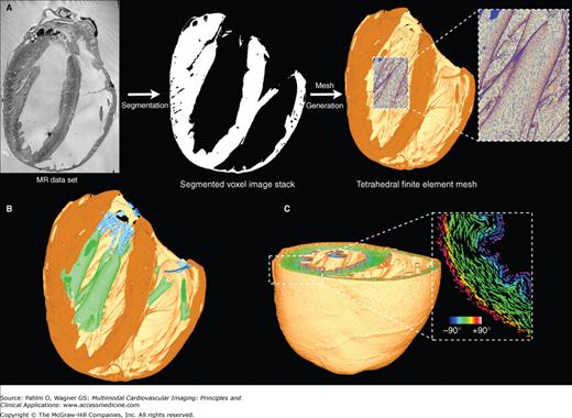
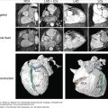
A. Magnetic resonance (MR)-to-model pipeline. Left. Longitudinal slice from a high-resolution MR image of the rabbit still heart with resolution of approximately 25 μm isotropic.43 Center. Segmentation of the high-resolution MR data set to produce binary segmented voxel image stack with atria removed. Right. Generation of a high-resolution tetrahedral finite element mesh directly from segmented voxel stack. Highlighted region shows high quality of mesh representation of intricate endocardial surface structures. B. Visualization of tagged structures within the ventricular model showing papillary muscles (green) and valves (blue), generated via manually created masks prior to mesh generation. C. Visualization of fiber vectors incorporated into the finite element mesh using the minimum distance algorithm described in the “Assignment of Fibrous Architecture” section.
As a result of this recent increase in attainable resolution, anatomical MR imaging (MRI) is now capable of providing a wealth of information regarding fine-scaled cardiac structural complexity. Such MR data are currently allowing accurate identification of microscopic features such as the coronary vasculature, extracellular cleft spaces, and the free-running PS, as well as macroscopic structures such as trabeculations and papillary muscles. However, differentiation of different tissue types is often problematic in anatomical MR, due to the very similar signal intensities recorded from functionally different tissue regions of the preparation. Furthermore, information regarding the organization of cardiomyocytes into cardiac fibers44 and the laminar structure of the myocardial wall45 is unattainable with normal anatomic MRI.
Myocardial structural information is more commonly obtained using a variation on the conventional anatomical MR protocol, called diffusion tensor MRI (DT-MRI). In DT-MRI, the measurement of the preferential direction of water molecule diffusion can be directly related to the underlying fiber architecture of the sample. It has been shown that the primary eigenvector from the diffusion tensor data (representing the direction of greatest water diffusion) corresponds faithfully with the cardiomyocyte direction (commonly referred to as the fiber direction), being validated with histological measurements.46 Similar measurements also suggest that the tertiary eigenvector represents the sheet-normal direction, although this correlation is still controversially debated.47
Although recent advances in DT-MRI protocols have reduced voxel resolutions to approximately 100 μm isotropic for small mammalian hearts, this is still approximately an order of magnitude greater than corresponding anatomical scans,43 which can cause problems when combining information from the two modalities. Due to this relatively low resolution, partial volume effects at tissue boundaries can also result in significant inaccuracies in predicted fiber orientation in these regions, particularly evident at epicardial/endocardial surfaces. Such effects occur when edge voxels contain a significant proportion of nontissue (where diffusion is generally isotropic) within their boundaries, meaning that the signal from these voxels does not accurately represent the underlying tissue structure in these boundary regions. This can also prove problematic close to intramural blood vessel cavities and extracellular cleft regions. Furthermore, traditional DT-MRI techniques have difficulties resolving more than one prevailing cell alignment direction in any one voxel, which can cause inaccuracies in regions such as the papillary muscle insertion site on the endocardium or where the RV and LV meet close to the septum, sites where there is known to be an abrupt change in fiber orientation. However, the development of novel DT-MRI protocols, such as Q-ball imaging,48 have been shown in recent preliminary studies to be able to successfully locate these regions of “mixed” fiber vectors, building on the success of such techniques used previously in brain DT-MRI acquisition to delineate regions of neural fiber crossing.
Following the acquisition of high-resolution structural and functional imaging data sets, described earlier, such information must then be processed and transformed into a usable format to facilitate the generation of anatomically detailed computational cardiac models. One important aspect of this is that all relevant information regarding gross cardiac anatomy, histoarchitectural heterogeneity, and structural anisotropy acquired in the images must be successfully translated over to the final model, so far as resolution requirements permit. Second, the computational pipeline of technology established for the analysis and processing of the images, and the generation and parameterization of the models from the imaging data should be as automated as possible, minimizing manual interaction. The development of such an automated pipeline will facilitate its use alongside imaging atlas data sets to investigate the causal effect of intrapopulation heterogeneities on simulations of cardiac function.
Anatomical MR data are the most common imaging data currently being used to construct the geometric basis of computational cardiac models. The first stage of the MR-to-model pipeline is to faithfully extract all of the complex geometric information present in the MRIs, which can then be carried over and used in the computational model. This is done by the process of segmentation. Segmentation is a broad and widely used technique within medical image analysis that involves labeling voxels based on their association with different regions, objects, or boundaries within the image. In certain cases, this can be done manually, for example, a highly experienced physician may segment by hand a region of tumorous tissue within an MRI or computed tomography (CT) scan. Alternatively, computational algorithms can be developed and used, based on a priori knowledge of the image features, to automatically segment regions of interest within the image, ideally with little or no manual input. To generate a computational model from cardiac MRIs, our initial goal is simply to identify those voxels in the MR data set that belong to cardiac “tissue” and those that represent nontissue or “background.” The background medium is generally identified in an MR scan as the lighter areas within the ventricular and atrial cavities, blood vessel lumens, the extracellular cleft spaces, and the medium on the exterior of the heart surrounding the preparation. Successful discrimination between background and tissue translates the gray scale MRI data set into a binary black/white (0/1) image mask.
Segmentation of the high-resolution rabbit MR data set shown in Fig. 14–1A, left43 was conducted using a level-set segmentation approach. Level-set methods are based on a numerical regimen for tracking the evolution of contours and surfaces.49 The contour is embedded as the zero level set of a higher dimensional function [Ψ(X, t)], which can be evolved under the control of a differential equation. Extracting the zero level set Γ(X, t) = ((X, t) = 0) allows the contour to be obtained at any time. A generic level-set equation to compute the update of the solution Ψ is given by:
where A, P, and Z are the advection, propagation, and expansion terms, respectively. The scalar constants α, β, and γ weight the relative influence of each of the terms on the movement of the surface, and thus, Equation 14–1 represents a generic structure that can be adapted to the particular characteristics of the problem. Different level-set filters use different features of an image to govern the contour propagation (eg, explicit voxel intensity or local gradient values) and can thus be combined to provide robust segmentation algorithms. Combining level-set filters in a sequential pipeline can be beneficial to provide a good initialization for filters that are prone to get trapped in local minima of the related cost function in the iterative solution to Equation 14–1. Figure 14–1A shows the final segmented voxel image stack of the rabbit MR data set following segmentation using a level-set approach.43
The final stage in the segmentation process involves the delineation of the ventricles from the segmented binary voxel image stack to facilitate the generation of a purely ventricular computational model. This requirement is such that the presence of an insulating layer of connective tissue that separates the ventricles from the atria (the annulus fibrosus) precludes direct electrical conduction between atrial and ventricular tissue. As a result, ventricular computational models are developed to allow the study of ventricular electrical function in isolation from the atria. Segmentation of the ventricles was performed by manual selection of 20 to 30 points in every fifth long axis slice through the MR data set along the line believed to represent the atrioventricular border. Identification of such a line was often possible because the connective tissue annulus fibrosus appeared relatively darker than the surrounding myocardium in the MR data. A smooth surface was then fitted through the landmark points to define a 2D surface, dissecting the image volume; all tissue voxels residing above the plane were subsequently removed, leaving only the ventricular tissue beneath. Figure 14–1A (center) shows the final segmented ventricular voxel image stack with atrial tissue removed.
Following discrimination between tissue and nontissue types in the segmentation process described earlier, it is further necessary to classify tissue voxels. Classification is either based on a priori knowledge or on additional complementary image sources or features that can be used to further differentiate functional or anatomical properties, both between different tissue types and also within a particular tissue type. Identifying such differences allows variations in electrical, structural, and/or mechanical parameters to be assigned on a per-region basis to tissue throughout the model, which is vital for realistic simulations of heart function. Each voxel can have one or more classifications, and for each classification, a numerical “tag” is assigned to the voxel. Importantly, these numerical tags within the voxel image stack are retained throughout the meshing process (see later section “Mesh Generation“), becoming associated with individual finite elements that make up the computational model.
Regions may be tagged in order to assign different cellular electrical properties to different tissue types. For example, the free-running Purkinje fibers are known to have very different electrical membrane dynamics compared with normal ventricular cells, requiring the use of specialized Purkinje cell models within these structures. In addition, tags can be used to assign different structural properties to distinct regions of tissue. For example, the papillary muscles and larger trabeculae (in places where they are detached from the endocardial wall) have a very different fiber architecture than myocytes lying within the bulk of the myocardial wall, tending to align parallel to the axis of these cylindrical structures. In all of these cases, it is often not possible to discern these different regions directly from the MR data because there is usually little or no difference in voxel intensities or intensity gradients between different regions. Although it is feasible that specialized and specific shape and appearance models may be developed to segment some of these different regions (eg, the papillary muscles and free-running Purkinje fibers have very distinctive morphologies), often manually created masks are produced and convoluted with the segmented image stack to numerically tag individual regions. Such a procedure was adopted to manually delineate structures such as the papillary muscles/larger trabeculae and valves from the segmented rabbit MR data, as well as the specialized Purkinje conduction system. Figure 14–1B shows tagged regions in the finite element rabbit ventricular model of Fig. 14–A (right), delineating the papillary muscles (green) and the valves (blue). In addition, Fig. 14–2A shows the manual identification of Purkinje fibers and their respective junctions within the MRI stack. Figures 14–2B,C shows the incorporation of this information into the ventricular model, allowing the tagged Purkinje fibers to be identified with corresponding specialized electrical properties.
Figure 14–2.
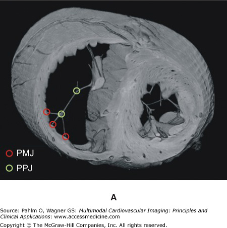
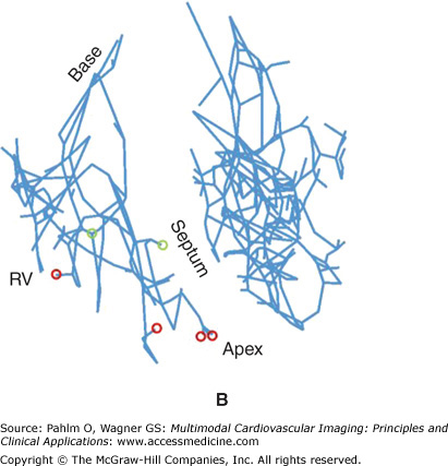
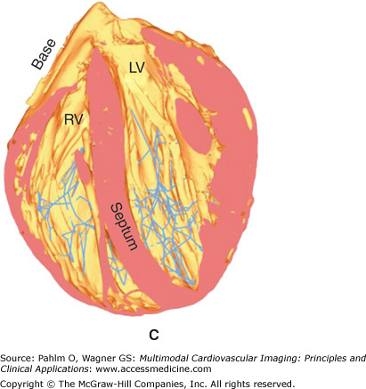
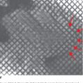
A. Manual identification of branching points within the free-running Purkinje system (Purkinje-Purkinje junctions [PPJ]) and points where the Purkinje fibers enter the myocardium (Purkinje-myocardial junctions [PMJ]) within the magnetic resonance image stack. B. and C. Corresponding delineation of Purkinje system within the computation ventricular model. LV, left ventricle; RV, right ventricle.
Furthermore, for certain applications, it may be required to delineate regions of diseased tissue, such as infarct, from the imaging data sets in order to assign the appropriate electrophysiological properties associated with such pathological conditions.50 Infarct tissue consists of both an inexcitable scar core and a border zone, which is assumed to contain excitable but pathologically remodeled tissue. Previous experimental studies have confirmed that myocardial necrosis, the influx of inflammatory cells with a more spherical morphology, and the deposition of collagen result in less anisotropic water diffusion within the infarct region as compared with healthy myocardium.51 Although scars cannot be discriminated from healthy myocardium in anatomical MR scans, the changes in diffusion anisotropy secondary to the structural remodeling are reflected in differences in fractional anisotropy values, which can be detected with DT-MRI scans.
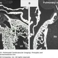
The image processing procedures to generate a model of an infarcted regions are presented in Fig. 14–3 using ex-vivo MRI and DT-MRI scans of a canine heart approximately 4 weeks after infarction.50 Using similar techniques as described earlier,49,52 the myocardium was separated from the surrounding suspension media and segmented to obtain an accurate representation of the anatomy. Similarly, the ventricles were separated from the rest of the myocardium to account for the presence of the electrically insulating annulus fibrosus as well as to assign different electrophysiological properties (atrial vs ventricular) to the tissue on either side of this boundary. After the delineation of the ventricles, the infarct tissue is labeled. From the interpolated DT-MRI, the fractional anisotropy (FA) image is generated by computing the FA of the diffusion tensor at each voxel.53 The FA of a diffusion tensor is defined as:
where λ1, λ2, and λ3 are the eigenvalues of the tensor. The FA is a measure of the directional diffusivity of water, and its values range from 0 to 1. A value of 0 indicates perfectly isotropic diffusion, and 1 indicates perfectly anisotropic diffusion. The infarct region is characterized by lower anisotropy, and therefore lower FA values, compared with the healthy myocardium51 because of the myocardial disorganization in the infarct. Based on this difference in FA values, the infarct region is separated from the normal myocardium by applying a level-set segmentation to the 3D FA image. Next, the infarct region is subdivided into two areas by thresholding the structural MRI based on the intensity values. It is observed in the MRIs that the infarct region has heterogeneous image intensities. This is due to the presence of two distinct regions within the infarct: a core scar, which is assumed to contain inexcitable scar tissue, and a peri-infarct zone (PZ), which is assumed to contain excitable but pathologically remodeled tissue. The two regions are separated by thresholding the structural MRI based on the intensity values of the voxels; regions of high (>75%) and low (<25%) gray-level intensities were segmented as core scar, whereas tissue of medium intensity was segmented as PZ.54,55 Figure 14–3 shows the final segmentation; orange identifies healthy myocardium, purple identifies the scar, and red identifies the PZ.
Alternatively, instead of a numerical tag, regions of the myocardium can be assigned quantitative information in the form of the value of a function at that particular point within the model. For example, the normalized transmural distance within the myocardial wall can be used to assign myocardial fiber orientation within the bulk of the myocardial wall (described later), as well as to modulate transmural gradients in electrophysiological cell membrane properties, with similar normalized distances used to modulate apico-basal electrophysiological cell membrane parameter gradients. Such functional parametrizations can be assigned to the voxel image stack, but are more commonly assigned on a per-node or per-element basis within the finite element mesh as a postprocessing step following modal generation, discussed later in the “Postprocessing” section.
Simulating the heart’s electrical or mechanical function requires that solution be sought to the different systems of equations that are used to model these aspects of cardiac behavior. In the case of tissue or whole organ simulations, it is required that the cardiac geometry in question be discretized into a set of grid or mesh points to facilitate a numerical solution approach to these equation systems. The majority of leading cardiac electrophysiology simulators (such as the one described later under “Simulating Cardiac Bioelectric Activity at the Tissue and Organ Level“) use finite element meshes as an input.56 However, the construction of finite element meshes, representative of the particular cardiac tissue/organ preparation, is a highly nontrivial task. Previously, direct experimental measurements from ventricular preparations have provided sets of evenly spaced node points, representing the external tissue surfaces, with finite elements subsequently being assigned joining up these points. Such procedures have been used in the construction of the widely used Auckland pig57 and canine58 ventricular models. Recently, finite element meshes have been constructed directly from anatomic imaging modalities, such as MR. Although the exceptionally high resolution of such data sets currently being obtained can provide unprecedented insight regarding intact cardiac anatomical structure, faithfully transferring this information into a finite element mesh that is both of good quality and computationally tractable is a significant challenge.
The mesh generation software of choice used by our group is Tarantula (http://www.meshing.at; CAE-Software Solutions, Eggenburg, Austria). Tarantula is an octree-based mesh generator that generates unstructured, boundary fitted, locally refined, conformal finite element meshes and has been custom designed for cardiac modeling. The underlying algorithm is similar to a recently published image-based unstructured mesh generation technique.59 Briefly, the method uses a modified dual mesh of an octree applied directly to segmented 3D image stacks. The algorithm operates fully automatically with no requirements for interactivity and generates accurate volume-preserving representations of arbitrarily complex geometries with smooth surfaces. The smooth nature of the surfaces ensures general applicability of the meshes generated, in particular for studies involving the application of strong external stimuli, because the smooth, unstructured grids lack jagged boundaries that can introduce spurious currents due to tip effects, as is the case for structured grids. To reduce the overall computational load of the meshes, unstructured grids can be generated adaptively such that the spatial resolution varies throughout the domain. Fine discretizations with little adaptivity can be used to model the myocardium, thus minimizing undesired effects of grid granularity on propagation velocity, while coarser elements that grow in size with distance from myocardial surfaces are generated to represent a surrounding volume conductor (eg, tissue bath or torso). Using adaptive mesh generation techniques facilitates the execution of bidomain simulations with a minimum of overhead due to the discretization of a surrounding volume conductor. Importantly with respect to model construction, Tarantula directly accepts the segmented voxel image stacks as input, which removes the need to generate tessellated representations of the cardiac surface, as required by Delaunay-based mesh generators.60 Avoiding this additional step is a distinct advantage in the development of high-throughput cardiac model generation pipeline.43
The final segmented and postprocessed data set was used to generate a tetrahedral finite element mesh using the meshing software Tarantula, shown in Fig. 14–1A. In addition to meshing the myocardial volume, a mesh of the volume conductor surrounding the ventricular mesh was also produced. This extracellular mesh not only consists of the space within the ventricular cavities and the vessels, but also defines an extended bath region outside of the heart, which can be used to model an in vitro situation where the heart is surrounded by a conductive bath, such as during optical mapping experiments.61 The total mesh produced by Tarantula shown in Fig. 14–1A consisted of 6,985,108 node points, making up 41,489,283 tetrahedral elements. The intracellular mesh consisted of 4,306,770 node points making up 24,199,055 tetrahedral elements with 1,061,480 bounding triangular faces. The myocardial mesh had a mean tetrahedral edge length of 125.7 μm. The mesh took 39 minutes to generate using two Intel Xeon processors, clocked with 2.66 GHz.43
Whenever possible, classification and tagging operations are carried out at the preprocessing stage prior to mesh generation. In general, it is much simpler to devise algorithms that operate on perfectly regular image data sets than on fully unstructured finite element meshes. Further, due to the large and very active medical imaging community, a vast number of powerful image- processing techniques are readily available through specialized toolkits.52 However, a subset of operations is better employed directly to the finite element mesh, because this is the computational grid that will be used for solving the biophysical problems. Although the objects, as defined by the binarized image stack on one hand and by the computational grid on the other hand, overlap fairly accurately, inevitable differences arise along the boundaries. The boundaries in the finite element mesh are smoothed representations of the object’s jagged boundaries in the voxel stack. Tags assigned on a per-voxel base prior to mesh generation have to be mapped over to the finite element mesh. This processing step, referred to as voxel mapping, is nonstandard and, as such, typically not an integral part of standard mesh generation software. Further, by using the finite element mesh, more complex tagging strategies can be conceived based on the use of the solution of partial differential equations (PDEs). An example is given in the following section, where a Laplace problem is solved on the finite element grid. The harmonic solution to the problem, φ, is then used to provide a reference frame for assigning tags. The scalar values of φ can be used as a measure of distance, for instance, the distance to the endocardium, and ∇φ may provide a reference that indicates the transmural direction at every node in the grid. An example of a postprocessing tag assignment is illustrated in Fig. 14–4. Here, it is shown how different regions within a ventricular finite element model may be tagged based on their locations relative to epicardial/endocardial surfaces, allowing epicardial, endocardial, and mid-myocardial regions to be defined. Depending on the tags held by different nodes within the mesh, different cellular ionic properties may be assigned to each region replicating the experimentally observed disparity in action potential dynamics seen within subepicardial/subendocardial/mid-myocardial regions of the ventricular walls. Another important postprocessing application is the regularization of DT-MRI data along the organ surfaces. DT-MRI data are very noisy and, due to partial volume effects, tend to be inaccurate close to surfaces. Such artifacts can be corrected easily by subtracting the projection of each fiber in surface elements onto the surface normal of the element from the fiber direction assigned to the element to ensure planarity of the fiber with the surface.
Figure 14–4.
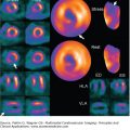
Tagging, consolidating, and assignment steps involved in the parametrization of biophysically detailed in silico models. Analysis of a ventricular finite element model (bottom left) provides information regarding a specialized intramural distance parameter (top left), which is then consolidated to delineate and tag within the mesh regions of the myocardial wall as subepicardial (1), mid-myocardial (2), and subendocardial (3) (top right). Such regions are then assigned different cellular ionic properties to allow experimentally observed variations in action potential dynamics to be reproduced (bottom right). This concept applies in a wider context and not only to the definition of transmural functional heterogeneity. Note that tags are assigned in a redundant manner to increase flexibility during the consolidation phase where new regions can be formed on the fly as a function of input parameters, allowing one to reuse in silico setups quickly while avoiding the time-consuming and error-prone tagging procedures. Parameters may be assigned on a per-node basis (as shown here for assigning models of cellular dynamics) or on a per-element basis (as suited for, eg, assigning tissue conductivities).
The specific arrangement of cardiac myocytes within the myocardium is known to highly influence the electromechanical functioning of the heart. Specifically, the orientation of cardiac fibers is responsible for the anisotropic conduction throughout the myocardium, with electrical conduction occurring more readily along the axis of the myofiber than in the plane normal to it. Furthermore, the preferential alignment of cardiomyocytes influences the mechanical functioning of the heart, with the development of active tension that causes contraction occurring solely parallel to the fiber direction. Therefore, a realistic representation of the fibrous architecture throughout the model is paramount to faithfully simulating cardiac behavior. From histological44 and DT-MRI46 analysis of cardiac fiber architecture, it is known that cardiac fibers run primarily in a circumferential (or latitudinal) direction through the myocardial wall, with an additional inclination in the apico-basal (or longitudinal) direction. The inclination, or helix, angle (α) varies transmurally by approximately 120° from epi- to endocardium, being approximately zero in the mid wall.27,44 In the following sections, we describe such experiment techniques used to measure fiber architecture within the heart, as well as mathematical rule-based methods for incorporating fiber information into cardiac models in the absence of experimentally measured data.
Information regarding cardiac fiber orientation can be obtained experimentally from either histological analysis42,62 or DT-MRI.46 Although the exceptional resolution of the histology data sets (up to approximately 1 μm in plane43) allows fiber orientation information to be readily extracted from the images through the application of simple gradient-based image analysis filters,42 a number of problems exist. First, the physical process of cutting the sample introduces significant nonrigid deformations to the tissue. Although it is possible to use the intact geometric information obtained from a prior anatomic MR scan to register the histology slices together to recover the correct intact anatomy,63 it is still unclear whether fully 3D information regarding cardiac fiber architecture can also be recovered from these registered data sets.
More commonly, myocardial structural information is obtained from DT-MRI recordings. Despite the potential drawbacks of DT-MRI, discussed earlier, the technique is widely used to embellish cardiac fiber orientation into computational models. There are two main ways in which DT-MRI information can be incorporated into an anatomical computational model. The first case is where the computational geometric model has been generated directly from a particular component of the DT-MRI data set; usually the intensity-based information, such as the FA or apparent diffusion coefficient values, is used. In these cases, the DT-MRI fiber vectors can be simply mapped across to the geometric finite element model using a nearest neighbor approach.64 However, the second case involves instances in which a computational model has been generated based on a previously obtained anatomical scan from the same sample, usually following reembedding in a medium with a different contrast agent required for the anatomical scan. Alternatively, a computational model is used that has been generated from a different preparation entirely and, in some cases, from a different species. Here, the two data sets need to be geometrically registered together prior to mapping.
However, in certain instances, such DT-MRI data sets are unavailable for a particular heart preparation. In these cases, fiber architecture can be embellished into the model through the use of rule-based approaches using a priori knowledge regarding cardiac fiber structure within the heart of a particular species. The two most commonly used rule-based methods are the minimum distance algorithm and the Laplace-Dirichlet method. Both methods involve defining a smoothly varying function throughout the tissue domain and then using information regarding the variation of the function to define fiber orientation vectors. Each method is now briefly described.
The minimum distance algorithm, developed by Potse et al,27 involves computing the minimum distance of every point within the myocardium to each of the epicardial (depi) and endocardial (dendo) surfaces, respectively. This is normally performed on a node-by-node basis over a finite element mesh, describing the tissue geometry. Within the septum, in absence of an epicardial surface, depi can be taken to be the minimum distance to the endocardial surface of the RV  , and dendo can be taken to be the minimum distance to the endocardial surface of the LV
  , replicating the apparent structural continuity of the LV and septum seen in previous imaging studies.46 With knowledge of depi and dendo, a normalized thickness parameter e is computed as:
To avoid sudden discontinuities in e at boundaries between regions, the value of e at each node is then averaged with all of its immediate neighbors (each central node of a structured mesh would have 26 neighbors). Calculation of the gradient of e within each tetrahedral element (∇e) then defines the transmural direction, u. The local circumferential direction, v, is then imposed to be perpendicular to u and the global apico-basal direction, which defines the “default” fiber vector direction with zero helix angle. To account for the widely reported transmural variation of fiber helix angle through the myocardial wall,44 a rotation of α is then made to the fiber vector about the u-axis. The most widely used functional representations of the variation of α through the wall are a linear or a cubic27 variation, which is the method adopted here, giving:
where eav was taken to be the average of e of the nodal values making up the tetrahedra. Due to the reportedly less pronounced variation of fiber angles in the LV compared with the RV, R is set equal to π/3 for the LV and septum and π/4 for the RV.27 Figure 14–1C shows the fiber vectors incorporated into the ventricular finite element model of Fig. 14–1A using the minimum distance approach.43
The Laplace-Dirichlet method involves computing the solution of an electric potential φ within the tissue between two electrodes:
where isotropic conduction within the tissue is assumed. Dirichlet boundary conditions specified at the electrode positions (one ground and the other fixed voltage) produce a smoothly varying potential field between the electrodes within the tissue. The resulting potential gradient vectors can then be used to assign smoothly aligned fiber vectors that align with the underlying global and local structure of the tissue. Smoothness along the boundaries is ensured because the electric field lines only originate/terminate at electrodes due to the zero-flux boundary condition specified on all other external tissue boundaries to simulate electrical isolation; thus, the field has no component perpendicular to the tissue boundary.
However, the Laplace-Dirichlet method is highly dependent on electrode configuration with respect to the specific tissue preparation. Electrodes can be placed to produce global apico-basal (longitudinal), transmural, or circumferential (latitudinal) field directions. Computation of the gradients of such fields within each finite element of the domain gives the local orthonormal basis vectors, from which the fiber vector can be assigned in a similar manner to the minimum distance approach discussed earlier.
In cases where vastly more complex geometric representations of the ventricles are constructed, simple rule-based methods cannot be used to faithfully assign fiber structure to all regions of the model. Such methods have been developed based on histological analysis of fiber vector architecture within the bulk of the ventricular free wall and therefore cannot be used to define fiber vectors in structures such as the papillary muscles or trabeculations, which are included within the next generation of cardiac models (as described earlier). Within such “tubular” endocardial structures, cardiac myocytes are known to align preferentially along the axis of the structure, because mechanically, this is the direction that facilitates the most efficient contraction. In such cases, the structure tensor method, a robust method for determining localized structure based on neighboring gradient fields, can be used to define local fiber orientation.
Simulating Cardiac Bioelectric Activity at the Tissue and Organ Level
Cardiac tissue is made up of myocytes of roughly cylindrical geometry. A myocyte is approximately 100 μm long and 10 to 20 μm in diameter. The intracellular spaces of adjacent myocytes are interconnected by specialized connexins referred to as gap junctions.65 The connexin expression over the cell is heterogeneous with a higher density of gap junctions at the intercalated discs located at the cell ends (along the long axis of the cell) and a lower density along the lateral boundaries,66,67 and different connexins of varying conductance are expressed in different regions of the heart.68 As a consequence of the elongated cellular geometry and the directionally varying gap junction density, current flows more readily along the longitudinal axes of the cells than transverse to it. This property is referred to as anisotropy. Cardiac tissue is composed of two spaces: an intracellular space formed by the interconnected network of myocytes, and the cleft space between myocytes referred to as interstitial space, which is made up of the extracellular matrix and the interstitial fluid. The extracellular matrix consists of networks of collagen fibers, which determine the passive mechanical properties of the myocardium. Electrically, it is assumed that the preferred directions are co-aligned between the two spaces but that the conductivity ratios between the principal axes are unequal between the two domains.38,69-71 All parameters influencing the electrical properties of the tissue, such as density and conductance of gap junctions, cellular geometry, orientation and cell packing density, and the composition of the interstitial space, are heterogeneous and may vary at all size scales, from the cellular level up to the organ. As a consequence, direction and speed of a propagating electric wave are constantly modified by interacting with discontinuous spatial variations in material properties at various size scales. At a finer size scale below the space constant, λ, of the tissue (ie, <1 mm), the tissue is best characterized as a discrete network in which the electrical impulse propagates in a discontinuous manner.72,73 At a larger more macroscopic size scale (>> λ), the tissue behaves as a continuous functional syncytium where the effects of small-scale discontinuities are assumed to play a minor role.
Theoretically, the idea of modeling an entire heart by using models of a single cell as the basic building block is conceivable. However, the associated computational costs are prohibitive with current computing hardware because a single heart consists of roughly 5 billion cells. Although a few high-resolution modeling studies have been conducted where small tissue preparations were discretized at a subcellular resolution,38,72,74 in general, the spatial discretization steps were chosen based on the spatial extent of electrical wave fronts and not on the size scales of the tissue’s microstructures. For this reason, cardiac tissue is treated as a continuum for which appropriate material parameters have to be determined that translate the discrete cellular matrix into an electrically analog macroscopic representation. In principle, this is achieved by averaging material properties over suitable length scales such that both potential and current solution match between homogenized and discrete representation. A rigorous mathematical framework for this procedure is provided by homogenization theory, which has been applied by several authors to the bidomain problem.15-75-77 Homogenization is a two-step process where the intracellular and interstitial domains are homogenized in a first step, and the two respective domains are spread out and overlapped to fill the entire tissue domain. This concept of interpenetrating domains states that everywhere within the entire myocardial volume intracellular space, extracellular space and the cellular membrane coexist.
The bidomain equations78 state that currents that enter the intracellular or extracellular spaces by crossing the cell membrane represent the sources for the intracellular, Φi, and extracellular potentials, Φe:
where σi and σe are the intracellular and extracellular conductivity tensors, respectively; β is the membrane surface-to-volume ratio; Im is the transmembrane current density; Itr is the current density of the transmembrane stimulus; Ie is the extracellularly applied current density; Cm is the membrane capacitance per unit area; Vm is the transmembrane voltage; and Iion is the density of the total current flowing through the membrane ionic channels, pumps, and exchangers, which in turn depends on the transmembrane voltage and a set of state variables η. At the tissue boundaries, electrical isolation is assumed, which is accounted for by imposing no-flux boundary conditions on Φe and Φi.
In those cases where cardiac tissue is surrounded by a conductive medium, such as blood in the ventricular cavities or a perfusing saline solution, an additional Poisson equation has to be solved:
Related posts:
 Optical Mapping of Electrical Activity
 Phonocardiography
 Ischemic Heart Disease
 Development of the Heart, with Particular Reference to the Cardiac Conduction Tissues
 Myocardial Perfusion Single Photon Emission Computed Tomography and Positron Emission Tomography
 Cardiac Magnetic Resonance Imaging in Ischemic Heart Disease
Stay updated, free articles. Join our Telegram channel

Full access? Get Clinical Tree


