Fig. 14.1
(a) A pretreatment PET scan of a head and neck cancer case of patient who died from disease after radiotherapy treatment. The head and neck tumor region of interest (brown) and the gross tumor volume (GTV) (green) were outlined by the physician. (b) an IVH plot, where Ix and Vx parameters are derived. (c) A texture map plot of the GTV heterogeneity through intensity spatial mapping
14.2.1.2 Dynamic Image Features
The dynamic features are extracted from time-varying acquisitions such as dynamic PET or MR. These features are based on kinetic analysis using tissue compartment models and parameters related to transport and binding rates (Watabe et al. 2006; Tofts 1997). Recently, using kinetic approaches, Thorwarth et al. published provocative data on the scatter of voxel-based measures of local perfusion and hypoxia in the head and neck (Thorwarth et al. 2006, 2007). Tumors showing widespread in both characteristics showed less reoxygenation during RT and had worse local control. An example from DCE-MRI is shown in Fig. 14.2, in which a three-compartment model is used and extracted parameters include the transfer constant (Ktrans), the extravascular-extracellular volume fraction (ve), and the blood volume (bv) (Sourbron and Buckley, Sourbron and Buckley 2011). A rather interesting approach to improve the robustness of such features is the use of advanced 4D iterative techniques (Reader et al. 2006). Further improvement could be achieved by utilizing multi-resolution transformations (e.g., wavelet transform) to stabilize kinetic parameter estimates spatially (Turkheimer et al. 2006).

Fig. 14.2
Dynamic features extracted from DCE-MRI in case of soft tissue sarcoma in the lower leg. Data are presented for two slices (top and bottom row, respectively), showing (a, f) slice position on a coronal T1-weighted image, (b, g) a fat-saturated high-resolution T2-weighted image of the slice with region-of-interest outlined, (c, h) the trans-endothelial transfer constant Ktrans (in 1/s), (d, i) the extravascular, extracellular space volume fraction ve (%), and (e, j) the blood volume fraction (bv) (%)
14.2.2 Outcome Modeling
Outcomes in radiation oncology are generally characterized by two metrics: tumor control probability (TCP) and the surrounding normal tissue complication probability (NTCP) (Steel 2002; Webb 2001). The dose-response explorer system (DREES) is a dedicated software tool for modeling of radiotherapy outcome (El Naqa et al. 2006c). A detailed review of outcome modeling in radiotherapy is presented in our previous work (El Naqa 2013). In the context of image-based treatment outcome modeling, the observed outcome (e.g., TCP or NTCP) is considered to be adequately captured by extracted image features (El Naqa et al. 2009; El-Naqa et al. 2004), where complementary imaging information are built into a data-driven model such as classical logistic regression approaches or more advanced machine learning techniques.
14.2.2.1 Outcome Modeling by Logistic Regression
Logistic modeling is a common tool for multi-metric modeling. In our previous work (Deasy and El Naqa 2007; El Naqa et al. 2006a), a logit transformation was used:

where n is the number of cases (patients), and x i is a vector of the input variable values (i.e., image features) used to predict f(x i ) for outcome y i (i.e., TCP or NTCP) of the i th:

(14.1)
(14.2)
where d is the number of model variables, and the β’s are the set of model coefficients determined by maximizing the probability that the data gave rise to the observations.
14.2.2.2 Outcome Modeling by Machine Learning
Machine learning represents a wide class of artificial intelligence techniques (e.g., neural networks, decision trees, support vector machines), which are able to emulate human intelligence by learning the surrounding environment from the given input data. These methods are increasingly being utilized in radiation oncology because of their ability to detect nonlinear patterns in the data (El Naqa et al. 2015a). This is due to their ability to detect complex patterns in heterogeneous datasets with superior results when compared to state of the art in each of these disciplines. In particular, neural networks were extensively investigated to model post-radiation treatment outcomes for cases of lung injury (Munley et al. 1999; Su et al. 2005) and biochemical failure and rectal bleeding in prostate cancer (Gulliford et al. 2004; Tomatis et al. 2012). A rather more robust approach of machine learning methods is kernel-based methods and its favorite technique of support vector machines (SVMs), which are universal constructive learning procedures based on the statistical learning theory (Vapnik 1998). Learning is defined in this context as estimating dependencies from data (Hastie et al. 2001).
There are two common types of learning: supervised and unsupervised. Supervised learning is used to estimate an unknown (input, output) mapping from known (input, output) samples (e.g., classification or regression). In unsupervised learning, only input samples are given to the learning system (e.g., clustering or dimensionality reduction). In image-based outcome modeling, we focus mainly on supervised learning, wherein the endpoints of the treatments such as TCP or NTCP are provided by experienced oncologists in our case.
For discrimination between patients who are at low risk versus patients who are at high risk of radiation therapy, the main idea of SVM would be to separate these two classes with “hyperplanes” that maximize the margin between them in the nonlinear feature space defined by implicit kernel mapping as shown in Fig. 14.3. The objective here is to minimize the bounds on the generalization error of a model on unseen data before rather than minimizing the mean-square error over the training dataset itself (data fitting). Mathematically, the optimization problem could be formulated as minimizing the following cost function:

subject to the constraint:

where wis a weighting vector and Φ(⋅)is a nonlinear mapping function. The ζ i represents the tolerance error allowed for each sample to be on the wrong side of the margin (called hinge loss). Note that minimization of the first term in Eq. (14.3) increases the separation (margin) between the two classes, whereas minimization of the second term improves fitting accuracy. The trade-off between complexity (or margin separation) and fitting error is controlled by the regularization parameter C. However, such a nonlinear formulation would suffer from the curse of dimensionality (i.e., the dimensions of the problem become too large to solve) (Haykin 1999; Hastie et al. 2001). Therefore, the dual optimization problem is solved instead of Eq. (14.3), which is convex complexity becomes dependent only on the number of samples and not on the dimensionality of the feature space. The prediction function in this case is characterized by only a subset of the training data, each of which are then known as “support vectors” s i :

where n s is the number of support vectors (i.e., samples at the boundary as in fig. 14.3), α i are the dual coefficients determined by quadratic programming, and K(⋅, ⋅) is the kernel function. Typical kernels (mapping functionals) include:

where c is a constant, q is the order of the polynomial, and σ is the width of the radial basis functions. Note that the kernel in these cases acts as a similarity function between sample points in the feature space. Moreover, kernels enjoy closure properties, i.e., one can create admissible composite kernels by weighted addition and multiplication of elementary kernels. This flexibility allows for the construction of a neural network by using a combination of sigmoidal kernels. Alternatively, one could choose a logistic regression equivalent kernel by proper choice of the objective function in Eq. (14.3). In Fig. 14.4, we show an example for the application of machine learning to predict local failure in lung cancer (El Naqa et al. 2010).


(14.3)
(14.4)
(14.5)
(14.6)
Fig. 14.3
Kernel-based mapping from a lower dimensional space (X) to a higher dimensional space (Z) called the feature space, where non-linearly separable classes become linearly separable
Fig. 14.4
Kernel-based modeling of TCP in lung cancer using gross tumor volume (GTV) and volume receiving 75 Gy (V75) with support vector machine (SVM) and a radial basis function (RBF) kernel. (a) Kernel-based modeling of TCP in lung cancer using the GTV volume and V75 with support vector machine (SVM) and a radial basis function (RBF) kernel. (a) Scatter plot of patient data (black dots) being superimposed with failure cases represented with red circles. Kernel parameter selection on leave-one-out cross-validation (LOO-CV) with peak predictive power attained at σ=2 and C=10,000. (b) Plot of the kernel-based local failure (1-TCP) nonlinear prediction model with four different risk regions: (1) area of low-risk patients with high confidence prediction level, (2) area of low-risk patients with lower confidence prediction level, (3) area of high-risk patients with lower confidence prediction level, and (4) area of high-risk patients with high confidence prediction level. Note that patients within the “margin” (cases ii and iii) represent intermediate-risk patients, which have border characteristics that could belong to either risk group. (c) A TCP comparison plot of different models as a function of patients’ being binned into equal groups using the model with highest predictive power (SVM-RBF). The SVM-RBF is compared to Poisson-based TCP, cEUD, and best two-parameter logistic model. It is noted that prediction of low-risk (high control) patients is quite similar; however, the SVM-RBF provides a significant superior performance in predicting high-risk (low control) patients
14.3 Radiomics Examples in Different Cancer Sites
In the following, we will provide two representative cases of image-based outcome modeling and discuss the processes involved in such development. In one case, we will use separate extracted features from PET and CT for predicting tumor control in lung cancer. In the other case, fused extracted features from PET and MR are used to predict distant metastasis to the lung in soft tissue sarcoma.
14.3.1 Predicting TCP in Lung Cancer
In a retrospective study of 30 non-small cell lung cancer (NSCLC) patients, 30 features were extracted from both PET and CT images with and without motion correction as shown in Fig. 14.5.

Fig. 14.5
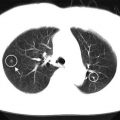
A pretreatment PET/CT scan of a lung cancer patient who failed locally after radiotherapy treatment. Top row shows scan samples in different views (transverse, sagittal, coronal). The bottom row shows the motion probability spread function (PSF) for not motion-corrected and motion-corrected (left to right)
The features included tumor volume; SUV/HU measurements, such as mean, minimum, maximum, and the standard deviation; IVH metrics; and texture-based features such as energy, contrast, local homogeneity, and entropy. The data corrected for motion artifacts based on a population-averaged probability spread function (PSF) using deconvolution methods derived from four 4D CT datasets (El Naqa et al. 2006b). An example of such features in this case is shown in Fig. 14.6.

Fig. 14.6
(a) Intensity volume histograms (IVH) of (b) CT and (b) PET, respectively. (c) and (d) are the texture maps of the corresponding region of interest for CT (intensity bins equal 100 HU) and PET (intensity bins equal 1 unit of SUV), respectively. Note the variability between CT and PET features: the PET-IVH and co-occurrence matrices show much greater heterogeneity for this patient. Importantly, patients vary widely in the amount of PET and CT gross disease image heterogeneity between patients
Using modeling approaches described in Sect. 14.2.2 and implemented in the DREES software, Fig. 14.7 shows the results for predicting local failure, which consisted of a model of two parameters from features from both PET and CT based on intensity volume histograms provided the best.

Fig. 14.7
 Computer-Assisted Treatment Planning Approaches for IMRT
 Computer-Aided Detection and Differentiation of Breast Cancer on Mammograms
 Computer-Aided Detection of Lung Cancer
 Computer-Assisted Treatment Planning Approaches for Carbon-Ion Beam Therapy
 Surface-Imaging-Based Patient Positioning in Radiation Therapy
 Computer-Assisted Target Volume Determination


Image-based modeling of local failure from PET/CT features. (a) Model order selection using leave-one-out cross-validation. (b) Most frequent model selection using bootstrap analysis where the y-axis represents the model selection frequency on resampled bootstrapped samples. (c) Plot of local failure probability as a function of patients binned into equal-size groups showing the model prediction of treatment failure risk and the original data (Reproduced with permission from Vaidya et al. 2012)
Related posts:
Computer-Assisted Treatment Planning Approaches for IMRT
Computer-Aided Detection and Differentiation of Breast Cancer on Mammograms
Computer-Aided Detection of Lung Cancer
Computer-Assisted Treatment Planning Approaches for Carbon-Ion Beam Therapy
Stay updated, free articles. Join our Telegram channel
Full access? Get Clinical Tree
