Diffusion MR Imaging: Basic Principles

From their origin as simple techniques primarily used for detecting acute cerebral ischemia, diffusion MR imaging techniques have rapidly evolved into a versatile set of tools that provide the only noninvasive means of characterizing brain microstructure and connectivity, becoming a mainstay of both clinical and investigational brain MR imaging. In this article, the basic principles required for understanding diffusion MR imaging techniques are reviewed with clinical neuroradiologists in mind.

Since the first descriptions of nuclear magnetic resonance (MR) in the 1950s, there has been interest in using MR to measure the diffusion properties of water. With the advent of MR imaging scanners in the 1980s, it was natural for investigators to develop diffusion MR imaging techniques for imaging of the brain, along the way demonstrating applications that are now familiar, such as restricted diffusion in acute cerebral ischemia and measurement of the directional dependence (anisotropy) of water diffusion in cerebral white matter. Once rapid single-shot echo planar imaging (SS-EPI) sequences became available in the early 1990s, diffusion MR imaging techniques were quickly adopted by many clinical radiologists and basic science investigators. As a result, there has been a rapid increase in knowledge of diffusion MR imaging techniques and their application to the study of brain pathology since that time: at last count, there were more than 8000 citations for brain diffusion MR imaging in the literature, approximately 2272 articles published in 2009 alone.

In this article, the basic principles required for understanding diffusion MR imaging techniques are reviewed with the clinical neuroradiologist in mind, setting the stage for detailed review of specific clinical applications in articles elsewhere in this issue. This article begins with a consideration of how diffusion MR imaging techniques exploit the random movements of water molecules to infer diffusion rates. It also considers the different methods for assessing anisotropic diffusion with emphasis on the most widely used model, known as diffusion tensor imaging (DTI). After reviewing current best practices in diffusion MR imaging acquisition, some of the common analytic methods used for diffusion MR imaging data are described, including advanced methods, such as tractography. Throughout, examples from the literature are used to illustrate the types of questions that can be addressed with diffusion techniques.

Physical basis of diffusion imaging

The Phenomenon of Brownian Motion

As commonly used in the physical sciences, the term, diffusion , carries two meanings. The classical meaning of the term refers to net molecular movement or flux down a concentration gradient. The Fick first law formalizes this concept and is familiar from medical school descriptions of respiratory physiology. Diffusion also refers, however, to the random displacement of molecules of uniform concentration in solution. This phenomenon is known as brownian motion, after the botanist Robert Brown, who noted its role in the displacement of pollen particles in solution.

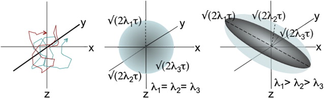
Brownian motion of water molecules is the key physical process that is measured in diffusion MR imaging experiments. According to theoretic models of brownian motion, the trajectory of a single molecule can be envisioned as a series of random collisions with surrounding molecules, all of which are agitated by thermal energy ( Fig. 1 ). Over time, any given molecule is displaced outward with radial location governed by a gaussian probability distribution (ie, a spherical shell with thickness determined by the variance of the gaussian distribution). Einstein is credited with formalizing this relationship by suggesting the mean squared displacement, < x ²>, from an initial point source takes the form (Equation 1 ):

< x 2 > = 6 D Δ t

where D is the diffusion constant/coefficient that is dependent on temperature, molecular size, and solvent viscosity, and Δ t represents the time elapsed from the initial position. Because the mean displacement, < x> , for a random process is zero, the variance (ie, square of the SD) is equal to this mean squared displacement. At physiologic temperatures, the constant D for water has a value of approximately 3 × 10 ³mm ²per second. Thus, over the 50- to 100-millisecond interval typically used in diffusion MR imaging experiments, the root mean squared displacement of water is on the order of a cell diameter, or approximately 10 mm.

The Diffusion MR Experiment

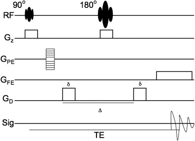
In the context of an imaging experiment, the challenge is to sensitize the MR signal to the diffusion of water (as described by Equation 1 ) while retaining the positional information used to identify each voxel in the image. In a typical pulsed gradient spin-echo diffusion-weighted sequence, this task is accomplished through the application of motion-sensitizing gradients just before and after the 180° refocusing pulse ( Fig. 2 ). Although the diffusion gradients are applied in the same direction in the MR pulse diagram, the effect of the gradients on spin phase is opposite because of the intervening refocusing/inversion pulse. Water protons that maintain their initial position between the application of the two gradient pulses experience no diffusion-related dephasing because the two lobes of the diffusion gradient negate each other. Diffusion away from the initial starting point, however, results in incomplete reversal of diffusion-related dephasing and proportionate loss of phase coherence (ie, signal). The loss of phase coherence is identical if the diffusion gradient is applied in the inverse direction (eg, the − x direction instead of the + x direction), and the aggregate behavior of the innumerable protons within any given voxel determines the degree of signal loss. Although the overall phase coherence is decreased by the presence of diffusion, the phase encoding itself remains unperturbed: the degree of phase offset by the phase-encoding gradient remains the same as for the diffusion gradient-free case, and the positional information is still recoverable by a standard 2-D Fourier transform.

This process has been formalized mathematically. First, it must be appreciated that the signal of any given voxel in a spin-echo sequence without a diffusion gradient takes the form as described in Equation 2 :

S o ∝ P D × ( 1 − e − T R / T 1 ) × e − T E / T 2

where PD is proton density, T1 and T2 are tissue properties, and echo time (TE) and repetition time (TR) are set by the instrument operator. These parameters are unchanged by the introduction of a diffusion gradient to the standard spin-echo sequence. There is exponential loss of signal (ie, dephasing), however, that occurs in the presence of a pulsed diffusion gradient, determined by the rate of diffusion in the direction of the diffusion gradient and strength/duration of the diffusion gradients. The relationship between the diffusion gradient, diffusion constant, initial signal, and diffusion-sensitized signal is described by the Stejskal-Tanner equation (Equation 3 ):

S n = S o × e − b × A D C n

where S _nrepresents the signal measured after application of a gradient in direction n , S _orepresents the intrinsic signal without diffusion gradients, and ADC _nis the apparent diffusion coefficient (ADC) of water in the direction of the applied gradient. The ADC is “apparent” in the sense that the diffusion constant may reflect macroscopic obstacles (eg, cell membranes or organelles) rather than the intrinsic mobility of water in the interrogated voxel. For this reason, the ADC in living tissues is typically lower than that measured for water solutions (discussed previously), approximately 1 × 10 ³mm ²/s. The value, b , is a measure of the diffusion weighting, factoring in both strength and duration of the diffusion gradient. For a typical, rectangular gradient pulse, it is defined as in Equation 4 :

b = γ 2 G 2 δ 2 ( Δ − δ 3 )

where γ represents the gyromagnetic ratio (1/(Tesla∗sec)), G the strength of the diffusion gradient (tesla/mm), δ the duration of the diffusion gradient (seconds), and Δ the interval between the start of each diffusion gradient (seconds). The units of b are seconds per m ², and typically b has values of 500 to 1000 s/mm ²in most clinical sequences.

From Equations 2–4 , diffusion MR imaging contrast (ie, difference between gradients on and off) is most efficiently increased through the application of strong diffusion gradients (G) that, therefore, result in large b values. Increasing the duration of the diffusion gradient (δ) also has a large effect on the b value and is another means of achieving sufficiently high diffusion weighting, although at the potential cost of increasing the TE. Increasing δ is most useful when operating near the Food and Drug Administration limitations placed on maximal gradient strength for human-rated MR scanners.

Solving for the ADC

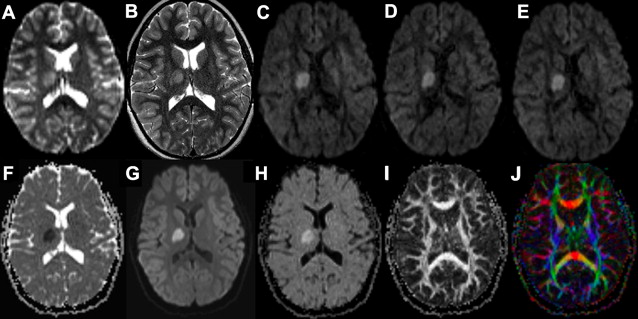
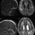
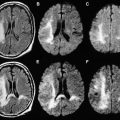
In Equation 3 , there are two unknown variables (S _oand ADC _n), one experimentally measured value (S _n), and one operator-specified value ( b ). Using basic algebra, the two unknown variables are readily solved by measuring S _nat two values of b , typically b = 0 and b = 1000 s/mm ²(eg, Fig. 3 A, C). Because b = 0 s/mm ²yields S _n= S _o, it is simple to solve for the ADC _nvalue (Equation 5 ):

A D C n = − ln ( S n / S o ) / ( b = 1000 s / m m 2 )

On some instruments, a third b value may be chosen between these two values to increase accuracy of the regression, but the concept is identical. One caveat to this calculation is that it assumes monoexponential decay of the diffusion-weighted signal, something that is not always observed in biologic specimens. There is usually an asymptotic deviation from monoexponential decay with large measured displacements (ie, b values), a phenomenon attributed to macromolecular barriers, such as cell membranes. At the b values typically encountered in a clinical diffusion MR imaging experiment, the deviations from monoexponential decay are relatively modest, but deviations from this assumption may have to be considered as diffusion gradient strength is increased, for example in diffusion spectrum imaging (DSI) or q-ball imaging (QBI) techniques ( Table 1 ). A second problem with calculations using Equation 5 is that it assumes isotropic diffusion of water throughout the brain. Because this is a fallacy in many regions of the brain (discussed later), it is standard practice to improve accuracy of the ADC measurement using values derived from 3 orthogonal directions, usually the X, Y, and Z axes relative to the scanner. Thus, the value of any given voxel in the ADC or diffusion-weighted images (DWI) reviewed by a radiologist represents the averaged values of at least 3 gradient directions (Equations 6 and 7 ):

A D C x y z = ( A D C x + A D C y + A D C z ) / 3

D W I x y z = S o × e − b × A D C x y z

Table 1

Imaging techniques

	DWI	DTI	QBI	DSI	Hemi– q -Space DSI	DKI
Encoding	SS-EPI-SE	SS-EPI-SE	SS-EPI-SE	2× Refocused SS-EPI-SE	SS-EPI-SE	2× Refocused SS-EPI-SE
Directions ^a	3	55	55	515 Points in q -space	129 Points in q -space	30
Matrix	160 × 136	128 × 128	128 × 128	128 × 128	112 × 112	128 × 128
Resolution	1.3 × 1.1 mm	1.8 × 1.8 mm	2.2 × 2.2 mm	2.0 × 2.0 mm	2.0 × 2.0 mm	2.0 × 2.0 mm
B Values (s/mm ²)	0, 500, 1000	1 q Radius (10) 1000	1 q Radius (30) 3000	5 q Radii, up to 17,000	5 q Radii, up to 12,000	0, 500, 1000, 1500, 2000, 2500
TE (ms)	92	63	82	154	89	108
TR (ms)	5500	14,000	16,400	3000	4200	2300
NEX	1	1	1	1	1	2
Acceleration Factor	1	2	2	NR	3	2
Acquisition Time (minutes)	30″	13′	16′	48′*	18′	12′
References

Abbreviations: NR, not reported; SE, spin echo; ∗, estimated from published acquisition parameters.

a Local protocol.

The ADC _xyzand DWI _xyzmeasurements from the 3-direction diffusion MR imaging experiment constitute the basic information available from a standard clinical MR sequence obtained for evaluation of stroke, and a study acquired in this way is referred to as a DWI experiment in this article.

The underlying SS-EPI spin-echo sequence is T2 weighted even on b = 1000 s/mm ²images where the cerebrospinal fluid signal is dephased due to diffusion effects (see Fig. 3 ). This T2 weighting is necessary because of the interval required for the application of the diffusion gradient (longer TE) and is valuable because it helps increase the conspicuity of lesions through combined effects of T2 and diffusion weighting. In instances where DWI signal is questioned as a shine-through artifact from the underlying T2 weighting, the T2 component can be removed computationally by dividing DWI _xyzby S _o, the latter representing the T2-weighted b = 0 s/mm ²image. The resulting (
D W I x y z / S o
) image is known as the exponential image (see Fig. 3 H).

Diffusion Anisotropy

In the basic DWI experiment (described previously), water is assumed to diffuse equally in all directions (ie, isotropically), something that is demonstrably false in many locations in the brain. The tendency of water to diffuse preferentially in certain directions is known as anisotropy and is highly correlated with the presence of coherent fiber bundles in brain tissue. Anisotropy was first demonstrated through comparison of ADC values obtained with application of diffusion gradients perpendicular to and parallel to long white matter tracts. The biophysical basis of this phenomenon remains somewhat uncertain. Measurements of unmyelinated neurons and neurons exposed to microtubule depolymerizing agents, however, still exhibit strong diffusion anisotropy, arguing against a primary role of the myelin sheath or cytoskeletal protein structure, respectively. Rather, much of the measured anisotropy is attributed to the cell membranes of the axons themselves. Therefore, anisotropic diffusion is commonly interpreted as coherent diffusion along the cell membranes of nerve fascicles as they traverse a voxel.

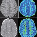
Because nerve fascicle orientation and trajectory cannot be noninvasively probed with any other method, measurement of diffusion anisotropy has attracted intense interest. The most widespread method for measuring diffusion anisotropy uses a model that assumes water diffusion at each voxel can be described by 3 orthogonal gaussian distributions with diffusion coefficients of magnitude λ ₁, λ ₂, and λ ₃. The relative magnitudes of the 3 diffusion coefficients determine the shape of the resulting probability distribution for water displacement/diffusion over the timescale of the applied diffusion gradient: if λ ₁= λ ₂= λ ₃, the diffusion probability distribution for the voxel is spherical; if λ ₁>> λ ₂, λ ₃, the probability distribution takes on an elongated/ellipsoid shape (see Fig. 1 , middle vs right panel). Because the set of 3 vectors (eigenvectors) corresponding to magnitudes λ ₁, λ ₂, and λ ₃(eigenvalues) specify a mathematical object known as a tensor, this model-based approach to measuring diffusion anisotropy is called DTI.

To determine the tensor for any given voxel, the diffusion coefficients along each of the 3 principal axes (X, Y, and Z) must be determined with respect to each of the other axes for a total of 9 values in a diffusion matrix:

[ D x x D x y D x z D y x D y y D y z D z x D z y D z z ]

Only gold members can continue reading. Log In or Register to continue