Dose Distribution and Scatter Analysis

It is seldom possible to measure dose distribution directly in patients treated with radiation. Data on dose distribution are almost entirely derived from measurements in phantoms—tissue-equivalent materials, usually large enough in volume to provide full-scatter conditions for the given beam. These basic data are used in a dose calculation system devised to predict dose distribution in an actual patient. This chapter deals with various quantities and concepts that are useful for this purpose.

9.1. Phantoms

Basic dose distribution data are usually measured in a water phantom, which closely approximates the radiation absorption and scattering properties of muscle and other soft tissues. Another reason for the choice of water as a phantom material is that it is universally available with reproducible radiation properties. A water phantom, however, poses some practical problems when used in conjunction with ion chambers and other detectors that are affected by water, unless they are designed to be waterproof. In most cases, however, the detector is encased in a thin plastic (water-equivalent) sleeve before immersion into the water phantom.

Since it is not always possible to put radiation detectors in water, solid dry phantoms have been developed as substitutes for water. Ideally, for a given material to be tissue or water equivalent, it must have the same effective atomic number, number of electrons per gram, and mass density. However, since the Compton effect is the most predominant mode of interaction for megavoltage photon beams in the clinical range, the necessary condition for water equivalence for such beams is the same electron density (number of electrons per cubic centimeter) as that of water.

The electron density (ρ_e) of a material may be calculated from its mass density (ρ_m) and its atomic composition according to the formula:

where:

N_A is Avogadro’s number and a_i is the fraction by weight of the ith element of atomic number Z_i and atomic weight A_i. Electron densities of various human tissues and body fluids have been calculated
according to Equation 9.1 by Shrimpton (1). Values for some tissues of dosimetric interest are listed in Table 5.1.

Table 9.1 Physical Properties of Various Phantom Materials

Material	Chemical Composition	Mass Density (g/cm³)	Number of Electrons/g (×10²³)	Z_eff^a (Photoelectric)
Water	H₂O	1	3.34	7.42
Polystyrene	(C₈H₈)_n	103–1.05	3.24	5.69
Plexiglas (Perspex, Lucite)	(C₅O₂H₈)_n	1.16–1.20	3.24	6.48
Polyethylene	(CH₂)_n	0.92	3.44	6.16
Paraffin	C_nH₂_n+₂	0.87–0.91	3.44	5.42
Mix D	Paraffin: 60.8
	Polyethylene: 30.4
	MgO: 6.4	0.99	3.41	7.05
	TiO₂: 2.4
M 3	Paraffin: 100
	MgO: 29.06	1.06	3.34	7.35
	CaCO₃: 0.94
Solid water^b	Epoxy resin-based mixture	1.00	3.34
^aZ_eff for photoelectric effect is given by Equation 6.4. ^bAvailable from Radiation Measurements, Inc. (Middleton, Wisconsin). Data are from Tubiana M, Dutreix J, Duterix A, et al. Bases physiques de la radiotherapie et de la radiobiologie. Paris: Masson ET Cie, Éditeurs; 1963:458; and Schulz RJ, Nath R. On the constancy in composition in polystyrene and polymethylmethacrylate plastics. Med Phys. 1979;6:153.

Table 9.1 gives the properties of various phantoms that have been frequently used for radiation dosimetry. Of the commercially available phantom materials, Lucite and polystyrene are most frequently used as dosimetry phantoms. Although the mass density of these materials may vary depending on a given sample, the atomic composition and the number of electrons per gram of these materials are sufficiently constant to warrant their use for high-energy photon and electron dosimetry.

In addition to the homogeneous phantoms, anthropomorphic phantoms are frequently used for clinical dosimetry. One such commercially available system, known as Alderson Rando Phantom,¹ incorporates materials to simulate various body tissues—muscle, bone, lung, and air cavities. The phantom is shaped into a human torso (Fig. 9.1) and is sectioned transversely into slices for dosimetric applications.

White et al. (2) have developed extensive recipes for tissue substitutes. The method is based on adding particulate fillers to epoxy resins to form a mixture with radiation properties closely approximating that of a particular tissue. The most important radiation properties in this regard are the mass attenuation coefficient, the mass energy absorption coefficient, electron mass stopping, and angular scattering power ratios. A detailed tabulation of tissue substitutes and their properties for all the body tissues is included in a report by the International Commission on Radiation Units and Measurements (3).

Based on the previous method, Constantinou et al. (4) designed an epoxy resin-based solid substitute for water, called solid water. This material could be used as a dosimetric calibration phantom for photon and electron beams in the radiation therapy energy range. Solid water phantoms are now commercially available from Radiation Measurements, Inc. (Middleton, WI).

9.2. Depth Dose Distribution

As the beam is incident on a patient (or a phantom), the absorbed dose in the patient varies with depth. This variation depends on many conditions: beam energy, depth, field size, distance from source, and beam collimation system. Thus, the calculation of dose in the patient involves considerations in regard to these parameters and others as they affect depth dose distribution. An essential step in the dose calculation system is to establish depth dose variation along the central axis of the beam. A number of quantities have been defined for this purpose, major among
these being percentage depth dose (5), tissue-air ratios (6,7,8,9), tissue-phantom ratios (10,11,12), and tissue-maximum ratios (12,13). These quantities are usually derived from measurements made in water phantoms using small ionization chambers. Although other dosimetry systems such as thermoluminescent dosimeters (TLD), diodes, and film are occasionally used, ion chambers are preferred because of their better precision and smaller energy dependence.

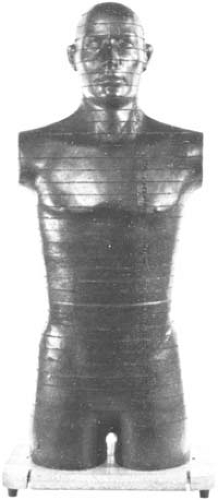Figure 9.1. An anthropomorphic phantom (Alderson Rando Phantom) sectioned transversely for dosimetric studies.

9.3. Percentage Depth Dose

One way of characterizing the central axis dose distribution is to normalize dose at depth with respect to dose at a reference depth. The quantity percentage (or simply percent) depth dose may be defined as the quotient, expressed as a percentage, of the absorbed dose at any depth d to the absorbed dose at a fixed reference depth d₀, along the central axis of the beam (Fig. 9.2). Percentage
depth dose (P) is thus:

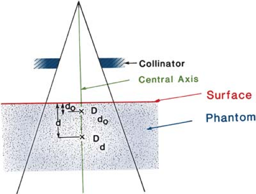Figure 9.2. Percentage depth dose is (D_d/D_d₀), where d is any depth and d₀ is reference depth of maximum dose.

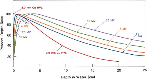Figure 9.3. Central axis depth dose distribution for different-quality photon beams. Field size, 10 × 10 cm; source to surface distance (SSD) = 100 cm for all beams except for 3.0 mm Cu half-value layer (HVL), SSD = 50 cm. (Data from Hospital Physicists’ Association. Central axis depth dose data for use in radiotherapy. Br J Radiol. 1978;[suppl 11]; and the Appendix.)

For orthovoltage (up to about 400 kVp) and lower-energy x-rays, the reference depth is usually the surface (d₀ = 0). For higher energies, the reference depth is taken at the position of the peak absorbed dose (d₀ =d_m).

In clinical practice, the peak absorbed dose on the central axis is sometimes called the maximum dose, the dose maximum, the given dose, or simply the D_max. Thus:

A number of parameters affect the central axis depth dose distribution. These include beam quality or energy, depth, field size and shape, source to surface distance, and beam collimation. A discussion of these parameters will now be presented.

A. Dependence on Beam Quality and Depth

The percentage depth dose (beyond the depth of maximum dose) increases with beam energy. Higher-energy beams have greater penetrating power and thus deliver a higher-percentage depth dose (Fig. 9.3). If the effects of inverse square law and scattering are not considered, the percentage depth dose variation with depth is governed approximately by exponential attenuation. Thus, the beam quality affects the percentage depth dose by virtue of the average attenuation coefficient

.² As the

decreases, the more penetrating the beam becomes, resulting in a higher-percentage depth dose at any given depth beyond the buildup region.

A.1. Initial Dose Buildup

As seen in Figure 9.3, the percentage depth dose decreases with depth beyond the depth of maximum dose. However, there is an initial buildup of dose that becomes more and more pronounced as the energy is increased. In the case of the orthovoltage or lower-energy x-rays, the dose builds up to a maximum on or very close to the surface. But for higher-energy beams, the point of maximum dose lies deeper into the tissue or phantom. The region between the surface and the point of maximum dose is called the dose buildup region.

The dose buildup effect of the higher-energy beams gives rise to what is clinically known as the skin-sparing effect. For megavoltage beams such as cobalt-60 and higher energies, the surface dose is
much smaller than the D_max. This offers a distinct advantage over the lower-energy beams for which the D_max occurs at the skin surface. Thus, in the case of the higher-energy photon beams, higher doses can be delivered to deep-seated tumors without exceeding the tolerance of the skin. This, of course, is possible because of both the higher percent depth dose at the tumor and the lower surface dose at the skin. This topic is discussed in greater detail in Chapter 13.

The physics of dose buildup may be explained as follows: (a) As the high-energy photon beam enters the patient or the phantom, high-speed electrons are ejected from the surface and the subsequent layers. (b) These electrons deposit their energy a significant distance away from their site of origin. (c) Because of (a) and (b), the electron fluence and hence the absorbed dose increase with depth until they reach a maximum. However, the photon energy fluence continuously decreases with depth and, as a result, the production of electrons also decreases with depth. The net effect is that beyond a certain depth the dose eventually begins to decrease with depth.

It may be instructive to explain the buildup phenomenon in terms of absorbed dose and a quantity known as kerma (from kinetic energy released in the μedium). As discussed in Chapter 8, the kerma (K) may be defined as “the quotient of dE_tr by dm, where dE_tr is the sum of the initial kinetic energies of all the charged ionizing particles (electrons) liberated by uncharged ionizing particles (photons) in a material of mass dm” (14):

Because kerma represents the energy transferred from photons to directly ionizing electrons, the kerma is maximum at the surface and decreases with depth because of the decrease in the photon energy fluence (Fig. 9.4). The absorbed dose, on the other hand, first increases with depth as the high-speed electrons ejected at various depths travel downstream. As a result, there is an electronic buildup with depth. However, as the dose depends on the electron fluence, it reaches a maximum at a depth approximately equal to the range of electrons in the medium. Beyond this depth, the dose decreases as kerma continues to decrease, resulting in a decrease in secondary electron production and hence a net decrease in electron fluence. As seen in Figure 9.4, the kerma curve is initially higher than the dose curve but falls below the dose curve beyond the buildup region. This effect is explained by the fact that the areas under the two curves taken to infinity must be the same.

B. Effect of Field Size and Shape

Field size may be specified either geometrically or dosimetrically. The geometric field size is defined as “the projection, on a plane perpendicular to the beam axis, of the distal end of the collimator as seen from the front center of the source” (15). This definition usually corresponds to the field defined by the light localizer, arranged as if a point source of light were located at the center of the front surface of the radiation source. The dosimetric, or the physical, field size is the distance intercepted by a given isodose curve (usually 50% isodose) on a plane perpendicular to the beam axis at a stated distance from the source.

Unless stated otherwise, the term field size in this book will denote geometric field size. In addition, the field size will be defined at a predetermined distance such as the source to surface distance
(SSD) or the source to axis distance (SAD). The latter term is the distance from the source to axis of gantry rotation known as the isocenter.

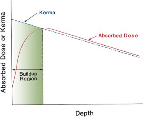Figure 9.4. Schematic plot of absorbed dose and kerma as functions of depth.

For a sufficiently small field one may assume that the depth dose at a point is effectively the result of the primary radiation, that is, the photons that have traversed the overlying medium without interacting. The contribution of the scattered photons to the depth dose in this case is negligibly small or 0. But as the field size is increased, the contribution of the scattered radiation to the absorbed dose increases. Because this increase in scattered dose is greater at larger depths than at the depth of D_max, the percent depth dose increases with increasing field size.

The increase in percent depth dose caused by increase in field size depends on beam quality. Since the scattering probability or cross section decreases with energy increase and the higher-energy photons are scattered more predominantly in the forward direction, the field size dependence of percent depth dose is less pronounced for the higher-energy than for the lower-energy beams.

Percent depth dose data for radiation therapy beams are usually tabulated for square fields. Since the majority of the treatments encountered in clinical practice require rectangular and irregularly shaped (blocked) fields, a system of equating square fields to different field shapes is required. Semiempirical methods have been developed to relate central axis depth dose data for square, rectangular, circular, and irregularly shaped fields. Although general methods (based on Clarkson’s principle—to be discussed later in this chapter) are available, simpler methods have been developed specifically for interrelating square, rectangular, and circular field data.

Day (16) and others (17,18) have shown that, for central axis depth dose distribution, a rectangular field may be approximated by an equivalent square or by an equivalent circle. Data for equivalent squares, taken from the Hospital Physicists’ Association (5), are given in Table 9.2. As an example, consider a 10 × 20-cm field. From Table 9.2, the equivalent square is 13.0 × 13.0 cm. Thus, the percent depth dose data for a 13 × 13-cm field (obtained from standard tables) may be applied as an approximation to the given 10 × 20-cm field.

A simple rule-of-thumb method has been developed by Sterling et al. (19) for equating rectangular and square fields. According to this rule, a rectangular field is equivalent to a square field if they have the same area/perimeter (A/P). For example, the 10 × 20-cm field has an A/P of 3.33. The square field that has the same A/P is 13.3 × 13.3 cm, a value very close to that given in Table 9.2.

The following formulas are useful for quick calculation of the equivalent field parameters. For rectangular fields:

where a is field width and b is field length. For square fields, since a = b:

where a is the side of the square. From Equations 9.5 and 9.6, it is evident that the side of an equivalent square of a rectangular field is 4 × A/P. For example, a 10 × 15-cm field has an A/P of 3.0. Its equivalent square is 12 × 12 cm. This agrees closely with the value of 11.9 given in Table 9.2.

Only gold members can continue reading. Log In or Register to continue