Filters and Convolution

(1)

Department of Mathematics and Statistics, Villanova University, Villanova, PA, USA

Electronic supplementary material

The online version of this chapter (doi:10.1007/978-3-319-22665-1_7) contains supplementary material, which is available to authorized users.

7.1 Introduction

Of constant concern in the analysis of signals is the presence of noise, a term which here means more or less any effect that corrupts a signal. This corruption may arise from background radiation, stray signals that interfere with the main signal, errors in the measurement of the actual signal, or what have you. In order to remove the effects of noise and form a clearer picture of the actual signal, a filter is applied.

For a first example of a filter, consider that the noise present in a signal is often random. That means that the average amount of noise over time should be 0. Consider also that noise often has a high frequency, so the graph of the noise signal is fuzzy and jaggedy. That means that the amount of noise should average out to 0 over a fairly short time interval. So, let T > 0 be a positive real number and let f represent a noisy signal. For each fixed value of x, the average value of f over the interval x − T ≤ t ≤ x + T is given by

$\displaystyle{ f_{\mathrm{ave}}(x) = \frac{1} {2T}\,\int _{t=x-T}^{x+T}f(t)\,dt. }$

(7.1)

The function f _ave that has just been defined represents a filtered version of the original signal f. For an appropriate value of T, the noise should average out to 0 over the interval, so f _ave would be close to the noise-free signal that we are trying to recover. If the value of T is too large, then some interesting features of the true signal may get smoothed out too much. If the choice of T is too small, then the time interval may be too short for the randomized noise to average out to 0.

A deeper analysis of (7.1) suggests that we consider the function $\,\phi = \sqcap _{T}/(2T)\,$ , where

$$$\displaystyle{ \sqcap _{T}(t) = \left \{\begin{array}{cc} 1&\mbox{ if $ - T \leq t \leq T$,}\\ 0 & \mbox{ if $\vert t\vert> T$.} \end{array} \right. }$$ ” src=”/wp-content/uploads/2016/10/A183987_2_En_7_Chapter_Equ2.gif”></DIV></DIV><br /> <DIV class=EquationNumber>(7.2)</DIV></DIV></DIV><br /> <DIV class=Para>Notice that<br /> <DIV id=Equa class=Equation><br /> <DIV class=EquationContent><br /> <DIV class=MediaObject><IMG alt=$

Also, for each fixed value of x, we get

$\displaystyle{ \phi (x-t) = \left \{\begin{array}{cc} \frac{1} {2T} &\mbox{ if $x - T \leq t \leq x + T$,}\\ 0 & \mbox{ otherwise.} \end{array} \right. }$

(7.3)

Hence, for any given function f and any fixed value of x, we get

$\displaystyle{ f(t)\,\phi (x-t) = \left \{\begin{array}{cc} \frac{1} {2T}\,f(t)&\mbox{ if $x - T \leq t \leq x + T$,}\\ 0 & \mbox{ otherwise,} \end{array} \right. }$

(7.4)

from which it follows that the integral in (7.1) is the same as the integral

$\displaystyle{ f_{\mathrm{ave}}(x) =\int _{ t=-\infty }^{\infty }f(t)\,\phi (x - t)\,dt. }$

(7.5)

Computationally, the function f _ave represents a moving average of the value of f over intervals of width 2T . This technique is used for the analysis of all sorts of signals — radio, electrical, microwave, audio — and also for things we might not think of as being signals, like long-term behavior of stock market prices.

Graphically, the graph of ϕ(x − t) as a function of t is obtained by flipping the graph of ϕ over from right to left and then sliding this flipped graph along the t-axis until it is centered at x instead of at 0 . This reflected-and-translated version of ϕ is then superimposed on the graph of f , and the area under the graph of the resulting product is computed. To generate the graph of f _ave , we reflect the graph of ϕ and then slide the reflected graph across the graph of f , stopping at each x value to compute the area underneath the product where the graphs overlap.

Example 7.1.

Consider a simple square wave:

$$$\displaystyle{\,f(t) = \sqcap _{a}(t) = \left \{\begin{array}{cc} 1&\mbox{ if $\vert t\vert \leq a$,}\\ 0 &\mbox{ if $\vert t\vert> a$.} \end{array} \right.}$$ ” src=”/wp-content/uploads/2016/10/A183987_2_En_7_Chapter_Equb.gif”></DIV></DIV></DIV>Take <SPAN id=IEq2 class=InlineEquation><IMG alt=$ as above. Let’s also assume that a ≥ T.

For any given value of x , the product f(t) ⋅ ϕ(x − t) will vanish at values of t outside the intersection of the intervals x − T ≤ t ≤ x + T and − a ≤ t ≤ a . The value of the integral $\,\int _{t=-\infty }^{\infty }f(t) \cdot \phi (x - t)\,dt\,$ will be equal to the length of this overlap multiplied by 1∕(2T).

There are three sets of values of x to consider. First, if | x | > T + a , then it is impossible to have both | t | ≤ a and | x − t | ≤ T . So f(t) ⋅ ϕ(x − t) = 0 for all t in this case. Next, for x satisfying | x | ≤ a − T , we have both − a ≤ x − T and x + T ≤ a. Hence, f(t) ⋅ ϕ(x − t) = 1∕(2T) whenever x − T ≤ t ≤ x + T; therefore,

$\displaystyle{\int _{t=-\infty }^{\infty }f(t) \cdot \phi (x - t)\,dt =\int _{ t=x-T}^{x+T}\left ( \frac{1} {2T}\right )\,dt = 1\,.}$

Finally, consider x such that a − T ≤ | x | ≤ a + T . In this case, the intersection of the intervals [x − T, x + T] and [−a, a] is either the interval [x − T, a] or the interval [−a, x + T] , depending on whether x is positive or negative, respectively. In either event, this intersection is an interval of width a + T − | x | . Hence, for such x , we get

$\displaystyle{\int _{t=-\infty }^{\infty }f(t) \cdot \phi (x - t)\,dt = \frac{1} {2T} \cdot \left (a + T -\vert x\vert \right )\,.}$

Combining these cases, we have shown that the filtered function f _ave , as in (7.5), is given by

$$$\displaystyle{ f_{\mathrm{ave}}(x) = \left \{\begin{array}{cc} 1 & \mbox{ if $\vert x\vert \leq a - T$,} \\ \frac{1} {2T} \cdot \left (a + T -\vert x\vert \right )&\mbox{ if $a - T \leq \vert x\vert \leq a + T$,} \\ 0 & \mbox{ if $\vert x\vert> a + T$.} \end{array} \right. }$$ ” src=”/wp-content/uploads/2016/10/A183987_2_En_7_Chapter_Equ6.gif”></DIV></DIV><br /> <DIV class=EquationNumber>(7.6)</DIV></DIV></DIV><br /> <DIV class=Para>Figure <SPAN class=InternalRef><A href=$ 7.1 shows an example of this. We see that, where the graph of f is a box (square wave) on the interval [−a, a] , the graph of f _ave has been spread out over the interval [−a − T, a + T]. The sides of the graph of f _ave are no longer vertical but sloped, with slopes ± 1∕(2T). Instead of a signal that starts and ends abruptly, as with the box, the smoothed-out signal fades in and fades out more gradually. In the case where a = T , the box actually becomes a tent. Perhaps we can visualize filling a rectangular box with dry sand. When the box is turned upside down and lifted away, the pile of sand will lose its box shape as the edges collapse. In the extreme case, the pile of sand will collapse into a cone.

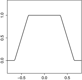
Fig. 7.1

The convolution of two boxes, in this case $\sqcap _{0.5}$ and $\sqcap _{0.15}$ , has the shape of a truncated tent. (If the boxes have the same width, then the convolution will be a tent.)

7.2 Convolution

When some other function g is used in place of $\,\sqcap _{T}/(2T)\,$ in the integral in (7.5), then the resulting function is not a simple moving average of the value of f over successive intervals. But we do get a modified version of f that has been “filtered” in a way that is determined by the function g. We make the following formal definition.

Definition 7.2.

Given two functions f and g (defined and integrable on the real line), the convolution of f and g is denoted by f ∗ g and defined by

$\displaystyle{ (f {\ast} g)(x):=\int _{ t=-\infty }^{\infty }f(t)\,g(x - t)\,dt\ \ \mathrm{for}\ x \in \mathbb{R}. }$

(7.7)

For instance, the function f _ave in (7.5) is the same as the convolution f ∗ϕ , where $\,\phi = \sqcap _{T}/(2T)\,$ . Graphically, the graph of f ∗ g can be obtained by reflecting the graph of g across the y-axis, then sliding the reflected graph across the graph of f , stopping at each x to compute the integral of the product where the two graphs overlap.

Example 7.3.

The formula for the convolution $\,\sqcap _{a} {\ast} (\sqcap _{T}/(2T))\,$ is given in (7.6).

Example 7.4.

For the tent function $$$\,\bigwedge (t) = \left \{\begin{array}{cc} 1 -\vert t\vert &\mbox{ if $ - 1 \leq t \leq 1$,}\\ 0 & \mbox{ if $\vert t\vert> 1$,} \end{array} \right.\,$$ ” src=”/wp-content/uploads/2016/10/A183987_2_En_7_Chapter_IEq10.gif”></SPAN> the convolution <SPAN id=IEq11 class=InlineEquation><IMG alt=$ is piecewise cubic on the interval − 2 ≤ x ≤ 2 and vanishes outside that interval.

In general, it is not so easy to compute the convolution of two functions by hand. The most manageable situation occurs if one of the functions is a box function $\,k \cdot \sqcap _{T}\,$ . Another helpful observation is that, if f vanishes outside the interval [a, b] and g vanishes outside the interval [c, d] , then the convolution f ∗ g vanishes outside the interval [a + c, b + d] . The proof of this is left as an exercise.

7.2.1 Some properties of convolution

Commutativity. For suitable functions f and g, we get

$\displaystyle{f {\ast} g = g {\ast} f.}$

Proof.

For each real number x , by definition

$\displaystyle{(f {\ast} g)(x) =\int _{ t=-\infty }^{\infty }f(t)\,g(x - t)\,dt.}$

Make a change of variables with u = x − t . Then du = −dt and t = (x − u) . Also, when t = −∞ , then u = ∞ and, when t = ∞ , then u = −∞ . (Remember that x is fixed throughout this process). Thus, the previous integral becomes

$\displaystyle{\int _{u=\infty }^{-\infty }f(x - u)\,g(u)\,(-du)}$

which is the same as the integral

$\displaystyle{\int _{u=-\infty }^{\infty }g(u)\,f(x - u)\,du.}$

This last integral is exactly the definition of (g ∗ f)(x) . Thus, f ∗ g = g ∗ f as claimed.

Linearity. For suitable functions f , g ₁ , and g ₂ , and for scalars α and β , we get

$\displaystyle{f {\ast} (\alpha g_{1} +\beta g_{2}) =\alpha (f {\ast} g_{1}) +\beta (f {\ast} g_{2}).}$

This property follows immediately from the fact that integration is linear. Combining this with the commutativity result, we also get that

$\displaystyle{(\alpha g_{1} +\beta g_{2}) {\ast} f =\alpha (g_{1} {\ast} f) +\beta (g_{2} {\ast} f).}$

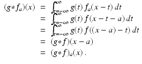
Shifting. Given a function f and a real number a , let f _a denote the shifted (translated) function

$\displaystyle{f_{a}(x) = f(x - a)\,.}$

Then, for suitable g , we get

$\displaystyle\begin{array}{rcl} (g {\ast} f_{a})(x)& =& \int _{t=-\infty }^{\infty }g(t)\,f_{ a}(x - t)\,dt {}\\ & =& \int _{t=-\infty }^{\infty }g(t)\,f(x - t - a)\,dt {}\\ & =& \int _{t=-\infty }^{\infty }g(t)\,f((x - a) - t)\,dt {}\\ & =& (g {\ast} f)(x - a) {}\\ & =& (g {\ast} f)_{a}(x)\,. {}\\ \end{array}$

Similarly,

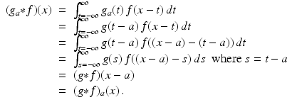
$\displaystyle\begin{array}{rcl} (g_{a} {\ast} f)(x)& =& \int _{t=-\infty }^{\infty }g_{ a}(t)\,f(x - t)\,dt {}\\ & =& \int _{t=-\infty }^{\infty }g(t - a)\,f(x - t)\,dt {}\\ & =& \int _{t=-\infty }^{\infty }g(t - a)\,f((x - a) - (t - a))\,dt {}\\ & =& \int _{s=-\infty }^{\infty }g(s)\,f((x - a) - s)\,ds\ \ \mathrm{where}\ s = t - a {}\\ & =& (g {\ast} f)(x - a) {}\\ & =& (g {\ast} f)_{a}(x)\,. {}\\ \end{array}$

Convolution with δ . The convolution of an arbitrary function with the Dirac delta function yields an interesting result — it isolates the value of the function at a specific point. Specifically, for each real number x , compute

$\displaystyle{(f{\ast}\delta )(x) =\int _{ t=-\infty }^{\infty }f(t)\,\delta (x - t)\,dt = f(x)\,,}$

where we have used the facts that δ(x − t) = 0 unless t = x and that $\,\int _{-\infty }^{\infty }\delta (s)\,ds = 1\,$ . In other words, convolution with δ acts like the identity map:

$\displaystyle{ (f{\ast}\delta )(x) = f(x)\ \ \mathrm{for\ all}\ x\,;\ \ f{\ast}\delta = f. }$

(7.8)

7.3 Filter resolution

The convolution of a function f with the δ function reproduces f exactly; so this filter has perfect resolution. More generally, let ϕ be a nonnegative function with a single maximum value M attained at x = 0. Suppose also that ϕ is increasing for x < 0 and decreasing for x > 0. (For example, ϕ could be a Gaussian or a tent.) Let the numbers x ₁ and x ₂ satisfy $x_{1} <0 <x_{2}$ and $\phi (x_{1}) =\phi (x_{2}) = M/2$ , half the maximum value of ϕ. The distance $(x_{2} - x_{1})$ is called the full width half maximum of the function ϕ, denoted FWHM(ϕ). For the filter of convolution with ϕ, the resolution of the filter is defined to be equal to FWHM(ϕ).

The idea is that a function ϕ having a smaller FWHM is pointier or spikier than a function with a larger FWHM and, hence, looks more like the δ function. So the resolution is better if the filter function ϕ has a smaller FWHM.

Here is a graphical way to see how the resolution of a filter is related to the FWHM of the filter function. Suppose a signal S consists of two impulses, two instantaneous blips, separated by a positive distance of a . Using the graphical approach to convolution, where we slide the reflected graph of the filter function ϕ across the graph of S , we see that, if a > FWHM(ϕ) , then the sliding copy of ϕ will slide past the first impulse before it really reaches the second one. Hence, the graph of (ϕ ∗ S) will have two distinct peaks, like S . But if a is less than FWHM(ϕ) , then the sliding copy of ϕ will overlap both impulses at once, so the two peaks will start to blend together. The detail in the original signal is getting blurry. For a sufficiently small, the graph of (ϕ ∗ S) will have only one peak, so the detail in S will have been lost completely. Overall, we see that the smallest distance between distinct features (the spikes) in the signal S that will still be distinct in the filtered signal (ϕ ∗ S) is a = FWHM(ϕ).

For a computational perspective, take a > 0 and let S be the signal S(x) = δ(x) +δ(x − a). Suppose also that the filter function ϕ is symmetric about x = 0 and achieves its maximum value M there. Thus, ϕ attains its half-maximum M∕2 when x = ±(1∕2) ⋅ FWHM(ϕ). Let’s also assume that the graph of ϕ tapers off fairly quickly away from 0, meaning that ϕ(x) ≈ 0 when | x | ≥ FWHM(ϕ). With this setup, the convolution is ϕ ∗ S(x) = ϕ(x) +ϕ(x − a), the sum of two copies of ϕ, one of which has been shifted to the right by a units. (Here we have used the shifting property of convolution together with formula (7.8) above.) So what happens if a = FWHM(ϕ)? Well, then we get ϕ ∗ S(a∕2) = ϕ(a∕2) +ϕ(−a∕2) = M∕2 + M∕2 = M. We also get ϕ ∗ S(0) = M +ϕ(−a) and ϕ ∗ S(a) = ϕ(a) + M, both of which are close to M in value, given our assumptions about the graph of ϕ . In other words, with a = FWHM(ϕ), the filtered signal (ϕ ∗ S) will be near M in value on the entire interval 0 ≤ x ≤ a. The two distinct spikes in S will get smeared or blurred across an interval. If a < FWHM(ϕ) , the blurring gets even worse. The detail in the signal has been lost! On the other hand, suppose a = 2 ⋅ FWHM(ϕ). Then ϕ will achieve its half-maximum value of M∕2 at ± a∕4. So ϕ ∗ S(0) = ϕ(0) +ϕ(−a) ≈ M and ϕ ∗ S(a) = ϕ(a) +ϕ(0) ≈ M. The filtered signal will have two distinct peaks, at or near x = 0 and x = a , with a valley in between, at x = a∕2. The original detail has been preserved.

Only gold members can continue reading. Log In or Register to continue