Flow Compensation and Modeling of IVIM MRI in the Liver and Pancreas

Joint Department of Physics, Institute of Cancer Research,15 Cotswold Rd, Sutton, Surrey, SM2 5NG, United Kingdom

andreas.wetscherek@icr.ac.uk

The combined use of flow-compensated and non-flow-compensated gradients in diffusion weighted MRI—aiming at separate charac- terization of diffusion and perfusion—is a natural choice from the perspective of Le Bihan’s original work [1]. In this chapter a brief history of flow-compensated IVIM in liver and pancreas is presented and the mathematical theory necessary to measure the characteris- tic timescale of the incoherent blood motion is derived. Experimental results indicate that the IVIM signal in the strongly perfused organs liver and pancreas cannot be fully understood within the commonly assumed pseudodiffusion limit and is closer to the microcirculatory straight-flow limit discussed in Ref. [2].

21.1 Introduction: History and Rationale of Flow-Compensated IVIM in Strongly Perfused Organs

“What is the characteristic timescale of the incoherent blood motion?” was the fundamental research question driving the work on IVIM in the group of Frederik Laun at the German Cancer Research Center (DKFZ) Heidelberg. Inspired by temporal diffusion spectroscopy [3], the first attempt to measure the characteristic timescale τ of the incoherent motion was to probe the perfusion spectrum D ^*(ω) with oscillating gradients. The core idea here is to rewrite the signal attenuation of the perfusion compartment as an integral over the product of gradient spectrum S(ω) and perfusion spectrum (Eq. 21.1). For details regarding this formalism see Ref. [4].

(21.1)

exp ( – b D ∗ ) → exp – γ 2 2 π ∫ – ∞ ∞ D ∗ ( ω ) S ( ω ) d ω

On the basis of Kennan’s derivation of the IVIM velocity autocorrelation function [5], τ could be characterized by the width of the central peak of D ^*(ω), which can be probed using sine and (flow-compensated) cosine gradients with different oscillation frequencies ω ₀ (Fig 21.1). It becomes apparent that this method is most sensitive for τω ₀ < 2π, which is equivalent to T ₀ > τ, with T ₀ denoting the oscillation period. As experimental results shown later in this chapter reveal, the characteristic timescale τ for pancreas and liver is of the order of a typical diffusion experiment, which would make very long echo times necessary to fit in several periods of oscillating diffusion gradients.

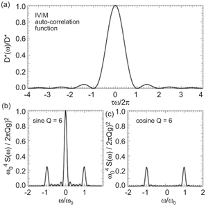
Figure 21.1 (a) IVIM autocorrelation function (perfusion spectrum) according to Ref. [5] and normalized gradient spectrum S(ω) for (b) sine and (c) cosine diffusion weighting with Q = 6 oscillations, oscillation frequency ω ₀, and gradient amplitude g.

The pursued solution was to effectively reduce the number of oscillations to 1 and rectify the waveform for increased diffusion weighting, which yielded the well-known Stejskal–Tanner [6] and the flow-compensated field even-echo refocusing (FEER) [7] waveform as the limits of sine and cosine, respectively. The first flow-compensated in vivo diffusion images of the abdomen must be attributed to Ahn et al., who calculated a difference image between those diffusion weightings, which was “believed to correspond to the capillary density map” [8]. Further analysis was performed by Maki et al., who detected perfusion changes in the rat brain with 10% CO₂ ventilation on the normalized difference image between flow-compensated and Stejskal–Tanner diffusion weighting [9]. Initial results obtained by combining those two diffusion weightings with echo-planar imaging showed a large signal difference in liver and pancreas between flow-compensated and non-flow- compensated gradients [10] but also revealed the susceptibility of the FEER diffusion-weighting scheme for artifacts originating from concomitant fields [11].

By introducing a flow-compensated diffusion weighting, which could be placed symmetrically around a refocusing pulse, concomi- tant field artifacts were effectively suppressed [12]. Figure 21.2 shows the symmetric monopolar and flow-compensated diffusion- weighting profiles and the definition of the diffusion time T used in this chapter. Being second-order motion compensated, the sym- metric flow-compensated profile was adopted in cardiac diffusion tensor imaging [13]. It allows for higher b values within the same preparation time than the M1M2 diffusion preparation introduced by Nguyen et al. [14].

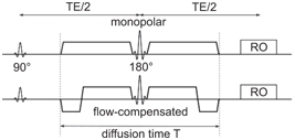
Figure 21.2 Symmetric monopolar and flow-compensated diffusion gradients and definition of the diffusion time T used in this chapter.

21.2 Theory

We start from the well-known IVIM signal equation (21.2),

S ( b ) = S 0 [ ( 1 – f ) e – b D + f e – b D b F ( b , T , v , τ ) ] ,

in which the attenuation of the tissue compartment with the fraction (1 – f) is described by the tissue’s apparent diffusion coefficient D. The perfusion compartment with the signal fraction f is attenuated both due to self-diffusion with the apparent diffusion coefficient of blood D _b and due to perfusion. While it was recently shown that the measured D _b depends on the hematocrit and the applied gradient waveform (because of a heavy exchange between red blood cells and plasma) [15], the attenuation F caused by blood flow is the focus of this theory section. For a more detailed derivation, the reader is directed to Refs. [12, 16].

In diffusion-weighted MRI, signal attenuation is caused by dephasing due to motion during the diffusion-weighting gradients. The signal attenuation F is therefore given by the phase distribution ρ(ϕ):

F = e i ϕ = ∫ – ∞ ∞ ρ ( ϕ ) e i ϕ d ϕ = ∫ – ∞ ∞ ρ ( ϑ ) e i ν ¯ b T υ d ϑ

Realizing that the accumulated phase ϕ scales with flow speed and gradient amplitude, a “normalized phase” ϑ was introduced [12], which is related to ϕ via ϕ = ν ¯ bT ϑ , where ν ¯ denotes the average blood flow velocity. It is left as an exercise to the reader to show that in this formalism a Gaussian distribution with N = T/τ corresponding to the number of directional changes during the diffusion experiment recovers the pseudodiffusion limit (Eq. 21.4a) and a uniform distribution with the width 1/ 3 represents straight flow (Eq. 21.4b), as discussed in Ref. [2]: