(1)
Intelligent Systems Research Centre, University of Ulster, Londonderry, UK
Abstract
This chapter presents a nonlinear system identification method (NSIM) for modeling effective connectivity for fMRI data analysis. We describe the theory background of the method and introduce the statistical tests for inferring effective connectivity between different brain regions. In addition, directional index is developed to quantify the information flow between these regions. However, applying NSIM method directly with nonlinear basis and high order of autoregression (AR) terms can lead to model overfitting problem. To circumvent this limitation, a model selection algorithm, i.e., a modified least-angle regression (MLARS), is employed to choose most significant nonlinear or linear covariates for mapping relationship between brain output (fMRI response) and input (experiment design). In the implementation of the MLARS method, Akaike’s information criterion corrected (AICc) algorithm was employed as a stop rule for model selection. As a result, the method builds model adaptively for different brain regions and overcomes the conventional method which needs a predefined structure/model for effective connectivity analysis.
Because of applying model selection algorithm at the first level data analysis, this leads to a new problem of bigger model variability for different runs/subjects to combine and compare at the group-level analysis. To overcome this limitation, we devise a robust regression method to examine model variability and label these extreme model parameters as outliers if they exceed certain threshold. Particularly, we employ a least-trimmed square robust method to remove these model outliers at group-level analysis.
Finally, we extend the NSIM for analyzing resting-state fMRI datasets. Because the nature of resting-state experiment, these data can be regarded as special cases where no system inputs are involved. Thus, NSIM can be applied without including system inputs as regression covariates. We give several examples to demonstrate how to use this method in studying effective connectivity.
Keywords
Effective connectivityModel selectionNonlinear system identificationRobust regressionResting-state fMRI (rfMRI)4.1 Nonlinear System Identification Method for fMRI Effective Connectivity Analysis
From brain integration viewpoint, all brain regions are connected with each other functionally or structurally, and from the angle of fMRI data analysis, brain connectivities can be roughly divided into three classes, i.e., structural, functional, and effective connectivities. Structural connectivity can be investigated by using diffusion weighted imaging as we will describe in Chap. 5. Functional connectivity is defined as the correlations between spatially remote neurophysiological events. This definition provides simple way to characterize functional interaction using correlation analysis and independent component analysis (ICA) methods. Since functional connectivity has been extensively studied, we will concentrate on introducing fMRI effective connectivity. In particular, we will focus on a model-free method, i.e., nonlinear system identification method (NSIM), to quantify effective connectivity (causality relationship) between different brain regions.
4.1.1 Current Methods for fMRI Effective Connectivity Analysis
Effective connectivity refers to the causality relationship between different brain regions, or one brain region influences another distant brain region. Generally, there are three approaches for modeling nonlinear brain activity in the study of functional magnetic resonance imaging (fMRI) effective connectivity. These methods can be categorized as white-box, gray-box, and black-box model methods [1]. White-box modeling is an off-building approach where the model is built before quantifying the connectivities. White-box modeling assumes that the structure of the neuron population is known, to address the problem of finding the parameters of the assumed structure. It is difficult to apply this identification method because the assumption of a known, stationary neuron population does not hold. Alternatively, gray-box models are often adopted when limited structural knowledge is available or assumed, and a model structure can be built on physical grounds, with a certain number of parameters to be estimated from the data. This could be a state-space model of a given order and structure. For example, using dynamic causal modeling (DCM) [2–5], an offline state-space model can be built at neuron level, and the effective connectivity can be studied by identifying the known structure of models corresponding to an infinitely precise prior on the model. A major limitation of this method is that it uses one offline model for all the brain regions without considering the variability of the fMRI response from different regions. For the black-box modeling method, the physical insight is not available or assumed, but the chosen model structure belongs to families that are known to have good flexibility and therefore can be adapted more easily to the data. Current black-box model approaches to study effective connectivity include the Granger causality model (GCM) [6–10], the (sparse) multivariate autoregression (MAR) model [11–13], and autoregression and moving average (ARMA) models [14]. These methods, however, do not include the experimental design as input for modeling the fMRI effective connectivity. This is not optimal when knowledge of the experimental design is available [2]. To circumvent this limitation, we have introduced a new nonlinear system identification method (black-box model method) for studying the effective connectivity [15]. We devised a scheme which identifies nonlinear connectivities using a nonlinear autoregressive exogenous model (NARX) method and provides statistics which can be used to test model interactions.
In this chapter, we firstly introduce the basic theory of NARX for fMRI effective connectivity analysis. Second, we show how the model is constructed for the investigation of nonlinear dynamic connectivity. In addition, we present the least squares algorithm to identify the strength of the various connectivities. Thirdly, we give an example of applying this method to the human visual system to study the brain region interactions. Fourthly, we extend this method for resting-state fMRI (rfMRI) data analysis. Finally, we introduce a robust statistical method for studying fMRI effective connectivity analysis at second-level data analysis.
4.1.2 Nonlinear System Identification Theory
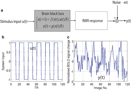
The nonlinear brain black box is depicted in Fig. 4.1a [5, 16, 17]. The input of the black box is the experimental design u(t) (Fig. 4.1b), and the output y(t) (Fig. 4.1c) is the fMRI response with some random noise e(t) added. Figure 4.1b is one example of a brain system input from phase-encoded and standard block designs. The system output or fMRI response y(t) is adaptively changed according to the input u(t) as shown in Fig. 4.1c. Formally, the physiological processes underlying the BOLD response can be modeled as a multiple-input and multiple-output (MIMO) system [16]:

and its discrete form is

where f and g are nonlinear functions and θ represents the set of model parameters. Under some mild assumptions, the discrete-time multivariate system (4.1) with p outputs (e.g., response from different regions) and q inputs (e.g., different types of stimuli) can be described by an autoregressive moving average with exogenous input (NARMAX) as follows [18, 19]:
![$$ \begin{array}{llllllll} y(t)={f}_g & \left[y\left(t-1\right),\dots, y\left(t-{n}_y\right),u\left(t-1\right),\dots, u\left(t-{n}_u\right), \right. \\ & \quad \left. e\left(t-1\right),\dots, e\left(t-{n}_e\right)\vphantom{y\left(t-{n}_y\right)}\right]+e(t) \end{array} $$](/wp-content/uploads/2016/04/A317179_1_En_4_Chapter_Equ3.gif)
where ![$$ y(t)=\left[\begin{array}{c}\hfill {y}_1(t)\hfill \\ \ \ \ \vdots \hfill \\ {}\hfill {y}_p(t)\hfill \end{array}\right] $$](/wp-content/uploads/2016/04/A317179_1_En_4_Chapter_IEq1.gif) ,
, ![$$ u(t)=\left[\begin{array}{c}\hfill {u}_1(t)\hfill \\ \vdots \hfill \\ {}\hfill {u}_q(t)\hfill \end{array}\right] $$](/wp-content/uploads/2016/04/A317179_1_En_4_Chapter_IEq2.gif) ,
, ![$$ e(t)=\left[\begin{array}{c}\hfill {e}_1(t)\hfill \\ \vdots \hfill \\ {}\hfill {e}_p(t)\hfill \end{array}\right] $$](/wp-content/uploads/2016/04/A317179_1_En_4_Chapter_IEq3.gif) are the system output, input, and noise, respectively; n y , n u , and n e are the maximum lags in the output, input, and noise; e(t) is a zero mean independent sequence; and f g is a new nonlinear function which can be obtained from nonlinear functions f and g. A special case of the general NARMAX model (4.3) is the nonlinear autoregressive with exogenous inputs (NARX) model which can be expressed as
are the system output, input, and noise, respectively; n y , n u , and n e are the maximum lags in the output, input, and noise; e(t) is a zero mean independent sequence; and f g is a new nonlinear function which can be obtained from nonlinear functions f and g. A special case of the general NARMAX model (4.3) is the nonlinear autoregressive with exogenous inputs (NARX) model which can be expressed as
![$$ y(t)={f}_g\left[y\left(t-1\right),\dots, y\left(t-{n}_y\right),u\left(t-1\right),\dots, u\left(t-{n}_u\right)\right]+e(t). $$](/wp-content/uploads/2016/04/A317179_1_En_4_Chapter_Equ4.gif)

Fig. 4.1
Nonlinear dynamic brain system for the phase-encoded experiment with 6 blocks (1 min/cycle). (a) Brain system block diagram; the gray box represents the nonlinear brain system. (b) Brain system input for standard block design or phase-encoded design. (c) Brain system output y(t) (fMRI response) curve for the corresponding boxcar function of the input u(t)

(4.1)

(4.2)
![$$ \begin{array}{llllllll} y(t)={f}_g & \left[y\left(t-1\right),\dots, y\left(t-{n}_y\right),u\left(t-1\right),\dots, u\left(t-{n}_u\right), \right. \\ & \quad \left. e\left(t-1\right),\dots, e\left(t-{n}_e\right)\vphantom{y\left(t-{n}_y\right)}\right]+e(t) \end{array} $$](/wp-content/uploads/2016/04/A317179_1_En_4_Chapter_Equ3.gif)
(4.3)
![$$ y(t)=\left[\begin{array}{c}\hfill {y}_1(t)\hfill \\ \ \ \ \vdots \hfill \\ {}\hfill {y}_p(t)\hfill \end{array}\right] $$](/wp-content/uploads/2016/04/A317179_1_En_4_Chapter_IEq1.gif) ,
, ![$$ u(t)=\left[\begin{array}{c}\hfill {u}_1(t)\hfill \\ \vdots \hfill \\ {}\hfill {u}_q(t)\hfill \end{array}\right] $$](/wp-content/uploads/2016/04/A317179_1_En_4_Chapter_IEq2.gif) ,
, ![$$ e(t)=\left[\begin{array}{c}\hfill {e}_1(t)\hfill \\ \vdots \hfill \\ {}\hfill {e}_p(t)\hfill \end{array}\right] $$](/wp-content/uploads/2016/04/A317179_1_En_4_Chapter_IEq3.gif) are the system output, input, and noise, respectively; n y , n u , and n e are the maximum lags in the output, input, and noise; e(t) is a zero mean independent sequence; and f g is a new nonlinear function which can be obtained from nonlinear functions f and g. A special case of the general NARMAX model (4.3) is the nonlinear autoregressive with exogenous inputs (NARX) model which can be expressed as
are the system output, input, and noise, respectively; n y , n u , and n e are the maximum lags in the output, input, and noise; e(t) is a zero mean independent sequence; and f g is a new nonlinear function which can be obtained from nonlinear functions f and g. A special case of the general NARMAX model (4.3) is the nonlinear autoregressive with exogenous inputs (NARX) model which can be expressed as![$$ y(t)={f}_g\left[y\left(t-1\right),\dots, y\left(t-{n}_y\right),u\left(t-1\right),\dots, u\left(t-{n}_u\right)\right]+e(t). $$](/wp-content/uploads/2016/04/A317179_1_En_4_Chapter_Equ4.gif)
(4.4)
By applying the regression equation, the NARMAX model (4.3) and NARX model (4.4) can be approximated as [20–22]

where P 0(t) = 1; for M ≥ 1, P m (t) = y 1 … y i u 1 u 2 … u j , i ≥ 1, j ≥ 0; m is the number of nonlinear terms; M is the system order; N is the total number of time point in the time series; i is the number of connected regions; and j is the number of inputs. Equation (4.5) denotes a general case where both input and output terms may be present, but it should be understood that some of the P m may contain only input or output terms and cross products. For example, for two stationary series of N values, the inputs  and y 2 and output y 1 of a closed-loop time-invariant nonlinear brain system can be described as [8]
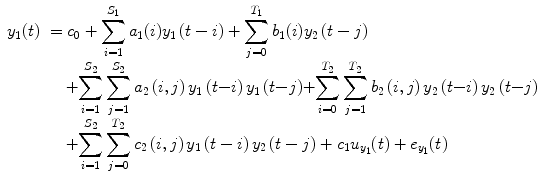
where the coefficients c 0, {a 1(i); b 1(j); c 1}, and {a 2(i, j); b 2(i, j); c 2(i, j)} denote constant (zeroth order), linear (first order), and nonlinear (second order) contributions to y 1(t), respectively.  represents the experimental input and
  is the prediction error of y 1(t). The model orders S 1 and S 2 are the maximum lags of the linear and nonlinear autoregressive (AR) influences, respectively, while the maximum lags for linear and nonlinear exogenous effects are determined by the model orders T 1 and T 2. The model can be represented in the matrix form as

where the vector Y = [y 1(1), y 2(2), … y 1(N)]T contains values of output series; ![$$ {e}_{y_1}=\left[{e}_{y_1}(1),{e}_{y_1}(2),\dots, {e}_{y_1}(N)\right] $$](/wp-content/uploads/2016/04/A317179_1_En_4_Chapter_IEq7.gif) is the prediction error series;
is the prediction error series; ![$$ {u}_{y_1}=\left[{u}_{y_1}(1),{u}_{y_1}(2),\dots, {u}_{y_1}(N)\right] $$](/wp-content/uploads/2016/04/A317179_1_En_4_Chapter_IEq8.gif) is the experimental input time series; A 1, B 1 and C 1 are the first-order vector coefficients; A 2, B 2, and C 2 are the second-order vector coefficients; and the matrices
is the experimental input time series; A 1, B 1 and C 1 are the first-order vector coefficients; A 2, B 2, and C 2 are the second-order vector coefficients; and the matrices  and
and  contain the S 1 linear AR terms and the (T 1 + 1) linear exogenous terms, respectively:
![$$ \begin{array}{llllllll} {H}_{y_1}&=\left[\arraycolsep3pt \begin{array}{cccc} {y}_1(0)\hfill & \hfill {y}_1\left(-1\right)\hfill & \hfill \cdots \hfill & \hfill {y}_1\left(1-{S}_1\right)\hfill \\ {y}_1(1)\hfill & \hfill {y}_1(0)\hfill & \hfill \cdots \hfill & \hfill {y}_1\left(2-{S}_1\right)\hfill \\ \vdots \hfill & \vdots \hfill & \hfill \hfill & \vdots \hfill \\ {y}_1\left(t-1\right)\hfill & \hfill {y}_1\left(t-2\right)\hfill & \hfill \hfill & \hfill {y}_1\left(t-{S}_1\right)\hfill \\ \vdots \hfill & \vdots \hfill & \hfill \cdots \hfill & \vdots \hfill \\ {y}_1\left(N-1\right)\hfill & \hfill {y}_1\left(N-2\right)\hfill & \hfill \cdots \hfill & \hfill {y}_1\left(N-{S}_1\right)\hfill \end{array}\right],\\ {H}_{y_2}&=\left[\arraycolsep3pt \begin{array}{cccc}\hfill {y}_2(1)\hfill & \hfill {y}_2(0)\hfill & \hfill \cdots \hfill & \hfill {y}_2\left(1-{T}_1\right)\hfill \\ {y}_2(2)\hfill & \hfill {y}_2(1)\hfill & \hfill \cdots \hfill & \hfill {y}_2\left(2-{T}_1\right)\hfill \\ \vdots \hfill & \vdots \hfill & \hfill \hfill & \vdots \hfill \\ {y}_2(t)\hfill & \hfill {y}_2\left(t-1\right)\hfill & \hfill \hfill & \hfill {y}_2\left(t-{T}_1\right)\hfill \\ \vdots \hfill & \vdots \hfill & \hfill \cdots \hfill & \vdots \hfill \\ {y}_2(N)\hfill & \hfill {y}_2\left(N-1\right)\hfill & \hfill \cdots \hfill & \hfill {y}_2\left(N-{T}_1\right)\hfill \end{array}\right], \end{array} $$](/wp-content/uploads/2016/04/A317179_1_En_4_Chapter_Equa.gif) the matrix
the matrix  contains the S 2(S 2 + 1)/2 quadratic AR terms given by the product of the terms of the matrix
  . In the same way, the matrix
  contains the (T 2 + 1)(T 2 + 2)/2 quadratic exogenous terms and the matrix
  contains the S 2(T 2 + 1) cross terms. Equation (4.7) can be written in the compact matrix format as

where ![$$ W=\left[{H}_1,{H}_{y_1},{H}_{y_2},{H}_{y_1{y}_1},{H}_{y_2{y}_2},{H}_{y_1{y}_2},{u}_{y_1}\right] $$](/wp-content/uploads/2016/04/A317179_1_En_4_Chapter_IEq15.gif) , β=[c 0, A 1T, B 1T, A 2T, B 2T, C 2T, c 1]T. Coefficient matrix β can be estimated by least squares:
, β=[c 0, A 1T, B 1T, A 2T, B 2T, C 2T, c 1]T. Coefficient matrix β can be estimated by least squares:

where pinv is the Moore–Penrose pseudoinverse of the matrix. By neglecting the nonlinear terms  and experimental input
  and considering only the first order of AR, i.e., AR(1), these lead to

or


(4.5)
 and y 2 and output y 1 of a closed-loop time-invariant nonlinear brain system can be described as [8]
(4.6)
 represents the experimental input and
  is the prediction error of y 1(t). The model orders S 1 and S 2 are the maximum lags of the linear and nonlinear autoregressive (AR) influences, respectively, while the maximum lags for linear and nonlinear exogenous effects are determined by the model orders T 1 and T 2. The model can be represented in the matrix form as
(4.7)
![$$ {e}_{y_1}=\left[{e}_{y_1}(1),{e}_{y_1}(2),\dots, {e}_{y_1}(N)\right] $$](/wp-content/uploads/2016/04/A317179_1_En_4_Chapter_IEq7.gif) is the prediction error series;
is the prediction error series; ![$$ {u}_{y_1}=\left[{u}_{y_1}(1),{u}_{y_1}(2),\dots, {u}_{y_1}(N)\right] $$](/wp-content/uploads/2016/04/A317179_1_En_4_Chapter_IEq8.gif) is the experimental input time series; A 1, B 1 and C 1 are the first-order vector coefficients; A 2, B 2, and C 2 are the second-order vector coefficients; and the matrices
is the experimental input time series; A 1, B 1 and C 1 are the first-order vector coefficients; A 2, B 2, and C 2 are the second-order vector coefficients; and the matrices  and
and  contain the S 1 linear AR terms and the (T 1 + 1) linear exogenous terms, respectively:
![$$ \begin{array}{llllllll} {H}_{y_1}&=\left[\arraycolsep3pt \begin{array}{cccc} {y}_1(0)\hfill & \hfill {y}_1\left(-1\right)\hfill & \hfill \cdots \hfill & \hfill {y}_1\left(1-{S}_1\right)\hfill \\ {y}_1(1)\hfill & \hfill {y}_1(0)\hfill & \hfill \cdots \hfill & \hfill {y}_1\left(2-{S}_1\right)\hfill \\ \vdots \hfill & \vdots \hfill & \hfill \hfill & \vdots \hfill \\ {y}_1\left(t-1\right)\hfill & \hfill {y}_1\left(t-2\right)\hfill & \hfill \hfill & \hfill {y}_1\left(t-{S}_1\right)\hfill \\ \vdots \hfill & \vdots \hfill & \hfill \cdots \hfill & \vdots \hfill \\ {y}_1\left(N-1\right)\hfill & \hfill {y}_1\left(N-2\right)\hfill & \hfill \cdots \hfill & \hfill {y}_1\left(N-{S}_1\right)\hfill \end{array}\right],\\ {H}_{y_2}&=\left[\arraycolsep3pt \begin{array}{cccc}\hfill {y}_2(1)\hfill & \hfill {y}_2(0)\hfill & \hfill \cdots \hfill & \hfill {y}_2\left(1-{T}_1\right)\hfill \\ {y}_2(2)\hfill & \hfill {y}_2(1)\hfill & \hfill \cdots \hfill & \hfill {y}_2\left(2-{T}_1\right)\hfill \\ \vdots \hfill & \vdots \hfill & \hfill \hfill & \vdots \hfill \\ {y}_2(t)\hfill & \hfill {y}_2\left(t-1\right)\hfill & \hfill \hfill & \hfill {y}_2\left(t-{T}_1\right)\hfill \\ \vdots \hfill & \vdots \hfill & \hfill \cdots \hfill & \vdots \hfill \\ {y}_2(N)\hfill & \hfill {y}_2\left(N-1\right)\hfill & \hfill \cdots \hfill & \hfill {y}_2\left(N-{T}_1\right)\hfill \end{array}\right], \end{array} $$](/wp-content/uploads/2016/04/A317179_1_En_4_Chapter_Equa.gif)
 contains the S 2(S 2 + 1)/2 quadratic AR terms given by the product of the terms of the matrix
  . In the same way, the matrix
  contains the (T 2 + 1)(T 2 + 2)/2 quadratic exogenous terms and the matrix
  contains the S 2(T 2 + 1) cross terms. Equation (4.7) can be written in the compact matrix format as
(4.8)
![$$ W=\left[{H}_1,{H}_{y_1},{H}_{y_2},{H}_{y_1{y}_1},{H}_{y_2{y}_2},{H}_{y_1{y}_2},{u}_{y_1}\right] $$](/wp-content/uploads/2016/04/A317179_1_En_4_Chapter_IEq15.gif) , β=[c 0, A 1T, B 1T, A 2T, B 2T, C 2T, c 1]T. Coefficient matrix β can be estimated by least squares:
, β=[c 0, A 1T, B 1T, A 2T, B 2T, C 2T, c 1]T. Coefficient matrix β can be estimated by least squares:
(4.9)
 and experimental input
  and considering only the first order of AR, i.e., AR(1), these lead to
(4.10)

(4.11)

(4.12)
This is the well-known two-connection linear GCM in fMRI data analysis.
4.1.3 Granger Causality (GC) Tests
Once the coefficients of the model are determined (e.g., Eq. (4.9)), Granger causality tests [6, 23, 24] are derived based on F/T statistics. For simplicity and illustrative purposes, we take the two-connection nonlinear models (4.6) as an example. The same principle can be applied for the linear system (Eqs. (4.11) and (4.12)). The tests for determining Granger causes (GC) are [23]:
1.
y 2 is GC of y 1 if b 1 = b 2 = c 2 = 0 in Eq. (4.6) is not true. Given the data, we reach this conclusion if b 1 = b 2 = c 2 = 0 is rejected.
2.
Similarly, y 1 Granger causes of y 2 can be investigated by reversing the input–output roles of the two series.
T and F statistics are developed to detect significant relations. From Eq. (4.8), and partitioning the coefficients as β = (β 1 : β 2) and W = (W 1 : W 2) accordingly, we can write this test as

with the maintained hypothesis. Therefore, T statistics given in Chap. 2 can be applied for testing the hypothesis. For the F-test, we employ the following equation:

where R in2 is the squared multiple correlation of the model containing all the variables in Eq. (4.8); R out2 is the squared multiple correlation from the reduced model with the term corresponding to β 2 = 0 removed, i.e., under null hypothesis; m is the number of terms corresponding to β 2, i.e., number of coefficients being jointly tested; k is the number of predictors in the full regression model, from which R in2 is derived; and n is the number of cases.

(4.13)

(4.14)
4.1.4 Directionality Indices
Directionality indices are quantified by computation of the absolute or relative predictability improvement obtained by the NARX model compared to the nonlinear autoregressive (NAR) model [8], i.e.,

where  represents the residual sum of square (RSS) from its own past (e.g., T 1 = T 2 = 0 in Eq. (4.6)) and RSS =
  .
.  denotes RSS for its own past and the past and present of the input series for a NARX model (e.g., T 1 ≠ 0, T 2 ≠ 0 in Eq. (4.6)). The relative causality index for the inputs y 2 and u 1 to the output y 1 is


(4.15)
 represents the residual sum of square (RSS) from its own past (e.g., T 1 = T 2 = 0 in Eq. (4.6)) and RSS =
  .
.  denotes RSS for its own past and the past and present of the input series for a NARX model (e.g., T 1 ≠ 0, T 2 ≠ 0 in Eq. (4.6)). The relative causality index for the inputs y 2 and u 1 to the output y 1 is
(4.16)
This index belongs to [0,1]. In the same way, the causality from input y 1 and u 2 to output y 2 can be investigated by reversing the input–output roles of the two series:


(4.17)

(4.18)
Finally, the relative strength of the causal interactions from y 2 to y 1 under influence of u 1 and u 2 is calculated by the directionality index:


(4.19)
 ranges from −1 to 1. A negative value implies that direction of causality is from y 2 to y 1, whereas a positive value indicates that the causality is from y 1 to y 2, and 0 means balanced bilateral interactions between y 2 and y 1.
4.1.5 Network Structure and Regional Time Series Extraction
To apply NSIM for fMRI effective connectivity study, the first step is to build the structure of brain network, although this step is not a requirement to apply NSIM method, because we can identify the system parameters and network structure using model selection method. The reason for using predefined brain network structure is because if we directly apply the method to the whole brain, we have to deal with the computational demanding problem, e.g., selecting the network structure from huge amount of voxels in the brain. If prior brain network structure can be obtained, it will greatly simplify the calculation. As an example for studying fMRI effective connectivity, we build the visual dorsal pathway network as displayed in Fig. 4.2.
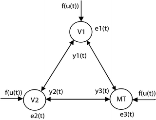

Fig. 4.2
3 connection dorsal visual network
Once the network has been constructed, we need to define the region of interests (ROI) from the brain image for the effective connectivity study. ROI can be defined by using standard template method or defined individually by stimulus-driven method. The later method is more accurate and considers individual variability, although it is time consuming to carry out this additional experiment. For instance, we can define the early visual cortex regions, i.e., V1–V4, by means of retinotopic mapping experiments. Because each brain’s ROI contains more than one fMRI time series, we need to choose one representative fMRI response from each ROI for connectivity study. There are two methods to select typical fMRI response for each region, e.g., random sample method and directly average method or using SVD method to average the time series within each region. For the random sample method, we can randomly select fMRI time series from the ROI and use it as representative response for the study. For the average method, we apply the singular value decomposition (SVD) method to get the representative time course for each ROI. In this method, assuming we have m time series (m voxels) in an ROI with n observations (fMRI image frames), we can form a matrix m × n matrix X and apply SVD method as
![$$ \left[U,S,V\right]=\mathrm{SVD}(X) $$](/wp-content/uploads/2016/04/A317179_1_En_4_Chapter_Equ20.gif)
where SVD is the MATLAB function, and then we keep the largest singular value S(1,1) and set all other elements in S to be 0. Then we do a reverse calculation to get the average representative signal Y as

![$$ \left[U,S,V\right]=\mathrm{SVD}(X) $$](/wp-content/uploads/2016/04/A317179_1_En_4_Chapter_Equ20.gif)
(4.20)

(4.21)
4.1.6 Examples to Apply NSIM to Study Effective Connectivity
To demonstrate how to use NSIM for effective connectivity study, we adopt the prior-defined dorsal visual network structure as shown in Fig. 4.2. We employ a random sample method to obtain the representative fMRI time course for each region from the retinotopic mapping experiment to overcome the limitation of averaging which can lead to blur the response delay. To use Eq. (4.5) for effective study, we need to select the order of nonlinearity and autoregression (AR) to model the nonlinear brain system. For reason of simplicity, although automatic AR order selection method is available to achieve this goal, we choose the nonlinearity of 2 and AR order of 1 for the study. Because the nonlinear system structure is defined (Fig. 4.2), we can apply Eq. (4.5) to calculate the system parameters. We employ the method to the retinotopic mapping data for one random selected run. The fMRI response (dotted curve) from V1, V2, and MT is displayed in Fig. 4.3b, d, f, respectively. Using Fourier transform method, we obtain the corresponding fundamental frequency (thin curve) as shown in Fig. 4.3a, c, e, respectively. Since system input (boxcar function denoted by the thick curves in Fig. 4.3a, c, e), output (dotted curves in Fig. 4.3b, d, f), and structure are determined, applying Eq. (4.9), we obtain system parameters as shown in the following equation:
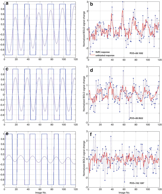

where u 1(t) (Fig. 4.3a), u 2(t) (Fig. 4.3c), and u 3(t) (Fig. 4.3e) are the system inputs. System output is displayed in Fig. 4.3b (y 1(t)), Fig. 4.3d (y 2(t)), and Fig. 4.3f (y 3(t)), respectively. Using the GC tests from Sect. 4.1.3, we calculate the F-test as shown in Table 4.1 for the fMRI time series in Fig. 4.3. In Table 4.1, 4.7106 is the V1 regional self-influence, 0.1604 denotes the regional influence from MT to V2, etc.

Fig. 4.3
Effective connectivity study. (a, c, and e) System inputs. (b, d, and f) System output and its prediction (using boxcar function as input)

(4.22)
Table 4.1
Causality test result using boxcar function as input
F-test, F(2,105) | V1(t) | V2(t) | MT(t) |
|---|---|---|---|
V1(t) | 4.7106 | 2.9397 | 1.8448 |
V2(t) | 0.1390 | 1.9178 | 0.1604 |
MT(t) | 2.1273 | 1.5353 | 0.1041 |
Based on Eqs. (4.15, 4.16, 4.17, 4.18, and 4.19), the directionality indices we obtained from V1 to V2 is 0.2562, from V2 to MT is 0.0584, and from MT to V1 is −0.3099. To investigate the input difference, we used the sinusoidal as shown in Fig. 4.3 (thin curve in Fig. 4.3a, c, e); the GC test results are given in Table 4.2. Similarly, the directionality indices we obtained from V1 to V2 is 0.2135; from V2 to MT is 0.2094, and from MT to V1 is −0.4048. Compare Table 4.1 with Table 4.2, we found that F values change using different input function. As we can see, the maximum influence is V1 self-influence in both tables, and the minimum influence is MT region self-influence using both boxcar function and sinusoidal function as inputs.


Table 4.2
Causality test result using sinusoidal function as input
F-test, F(2,106) | V1(t) | V2(t) | MT(t) |
|---|---|---|---|
V1(t) | 4.4450 | 3.1784 | 2.3019 |
V2(t) | 0.2507 | 1.4571 | 0.2397 |
MT(t) | 2.2114 | 1.0595 | 0.1194 |
Stay updated, free articles. Join our Telegram channel

Full access? Get Clinical Tree


