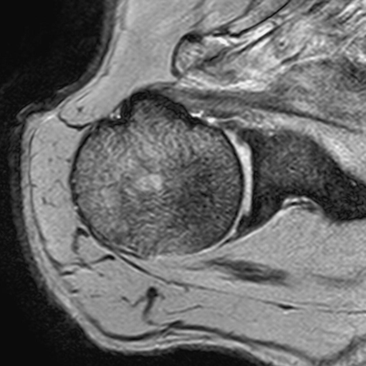
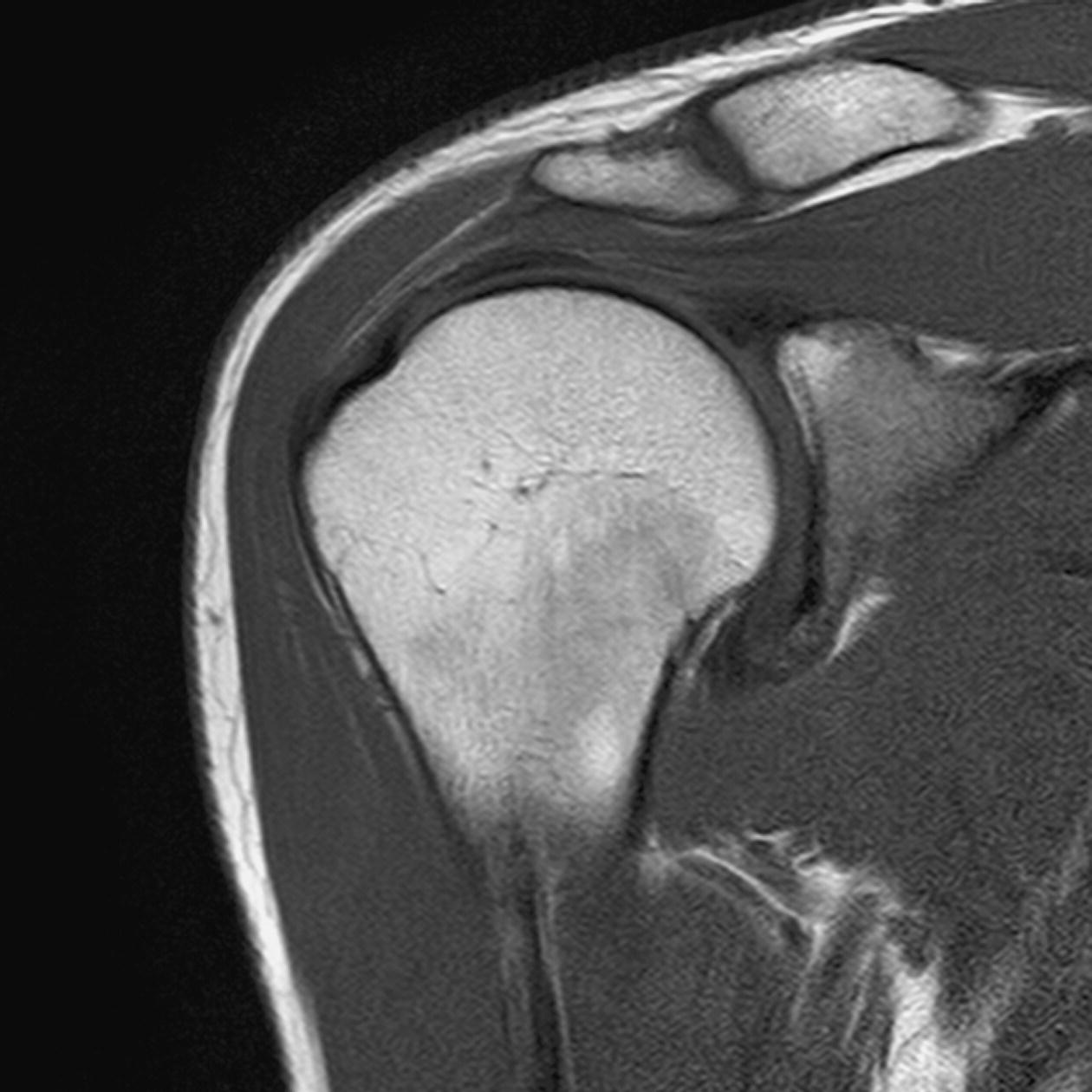
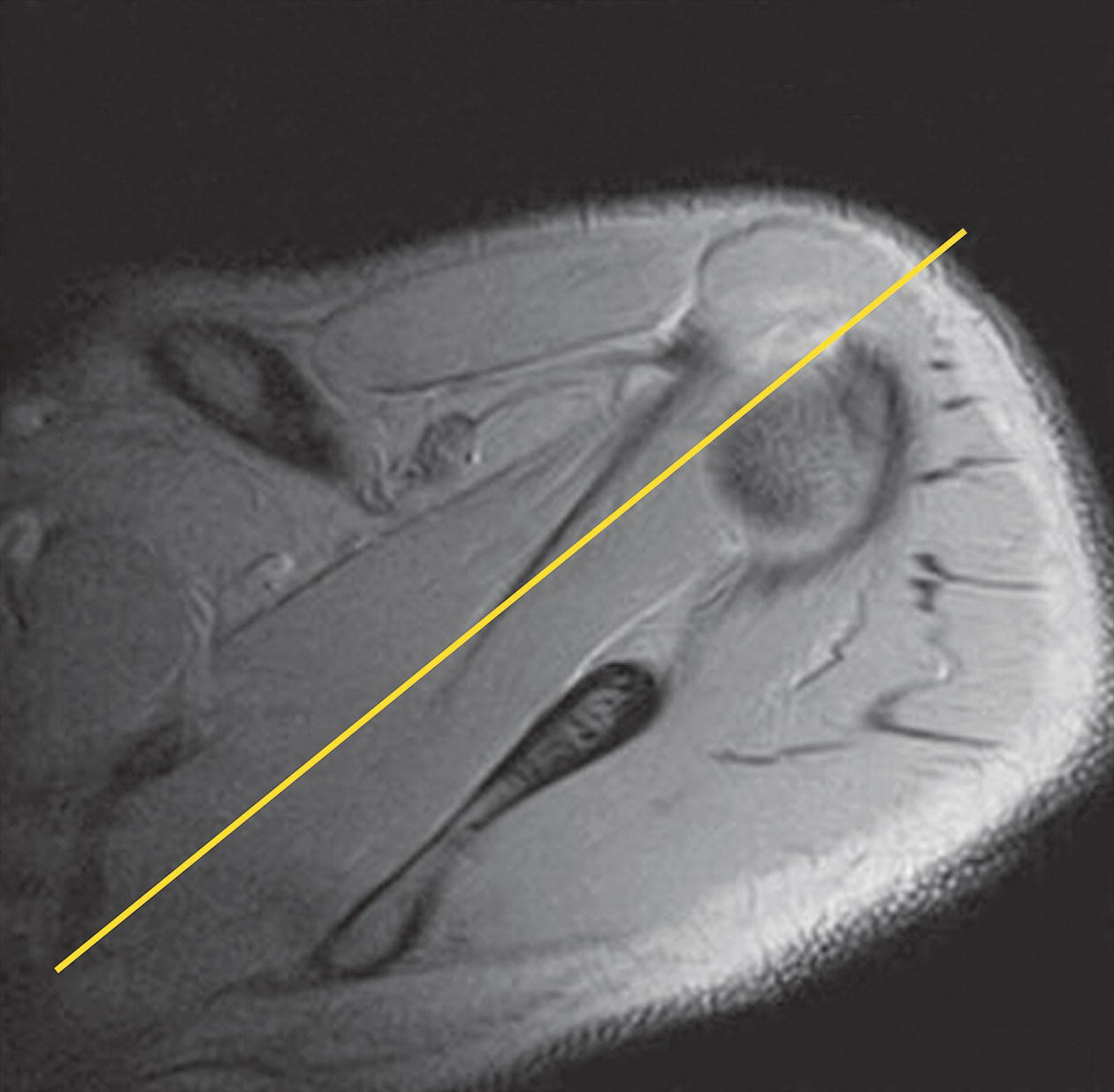
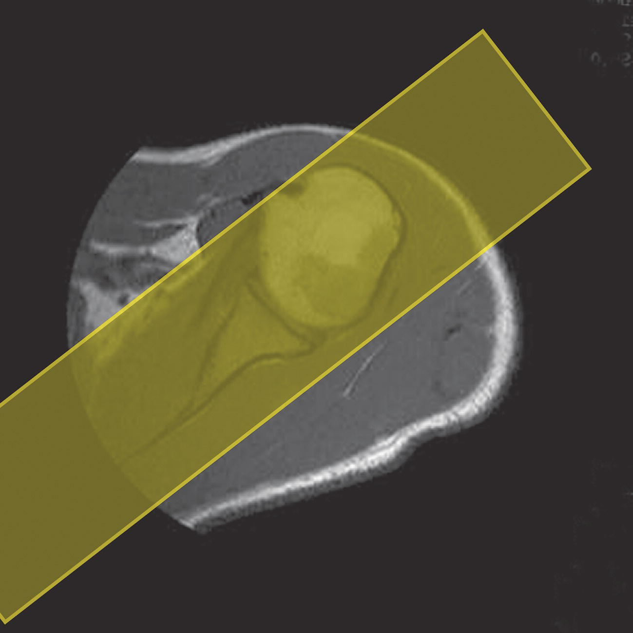
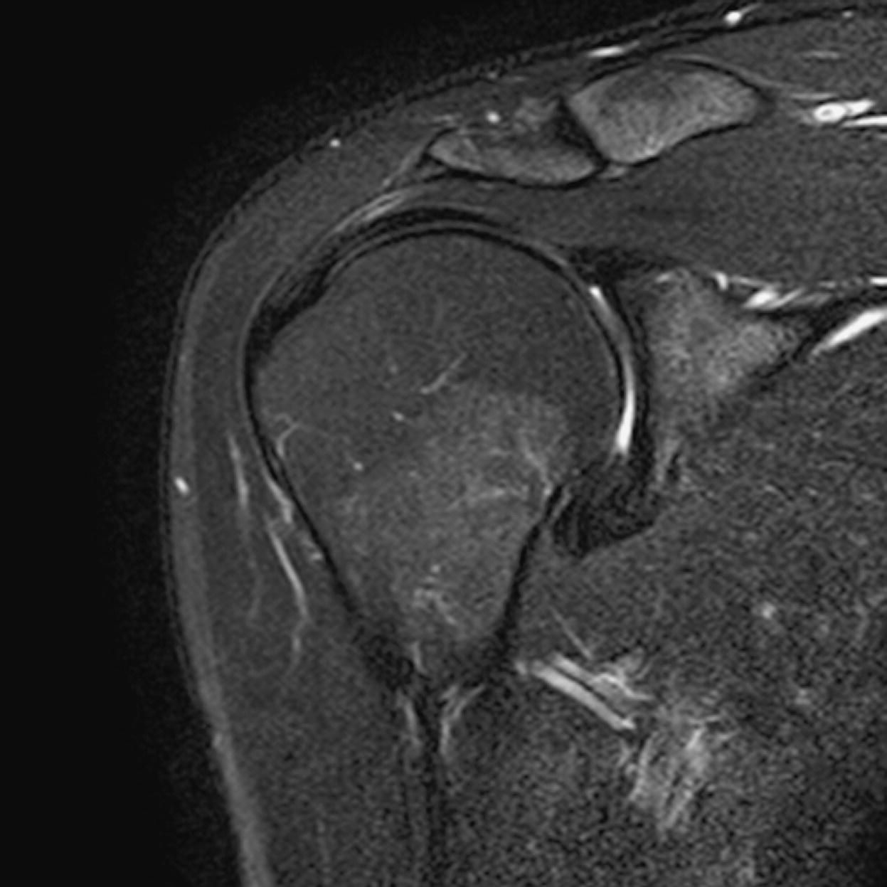
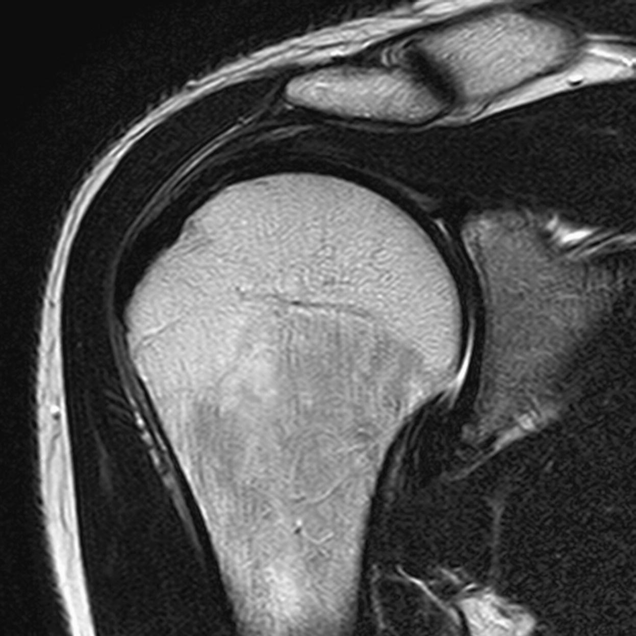
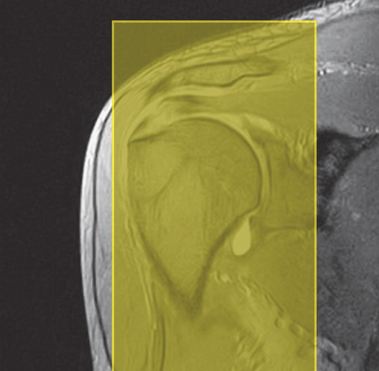
13 Table 13.1 Summary of parameters The figures given are for 1.5 T and 3 T systems. Parameters are dependent on field strength and may need adjustment for very low or very high field systems. Figure 13.1 Anterior view of the right shoulder showing bony structures and main ligaments. The patient lies supine with the arms resting comfortably by the side. Slide the patient across the table to bring the shoulder under examination as close as possible to the centre of the bore. Relax the shoulder to remove any upward ‘hunching’. The arm to be examined is strapped to the patient, with the thumb up (neutral position) and padded so that the humerus is horizontal. Place the coil to cover the humeral head and the anatomy superior and medial to it. If a surface or flexible coil is used, care must be taken to ensure that the flat surface of the coil is parallel to the Z axis when it is placed over the humeral head (Figure 1.1). Centre the FOV on the middle of the glenohumeral joint. Patient and coil immobilization are essential for a good result. If possible, instruct the patient to breathe abdominally rather than with the thorax and place sandbags on the upper chest. This reduces movement artefact. Instruct the patient not to move the hand during sequences. The patient is positioned so that the longitudinal alignment light and the horizontal alignment light pass through the shoulder joint. Acts as a localizer if three-plane localization is unavailable and ensures that there is adequate signal return from the whole joint. Medium slices/gaps are prescribed relative to the horizontal alignment light so that the supraspinatus muscle is included in the image. Axial localizer: I 0 mm to S 25 mm Figure 13.2 Axial GRE T2*-weighted image of the shoulder showing normal appearances. Thin slices/gaps are prescribed from the top of the acromio-clavicular joint to below the inferior edge of the glenoid (Figure 13.3). The bicipital groove on the lateral aspect of the humerus to the distal supraspinatus muscle is included in the image. The axial projection displays joint cartilage and glenoid labrum, intra-osseous changes associated with Hills–Sachs deformity, and the condition of muscles and tendons of the rotator cuff. Figure 13.3 Axial GRE T2*-weighted image showing slice prescription boundaries and orientation for axial imaging of the shoulder. Figure 13.4 Coronal/oblique T1-weighted FSE through the shoulder. Thin slices/gaps are prescribed from the infra-spinatus posteriorly to the supraspinatus anteriorly and angled parallel to the supraspinatus muscle (Figures 13.5 and 13.6). This is best seen on a superior axial view, but coverage is easier to assess on an axial image through the lower third of the humeral head. The superior edge of the acromion to the inferior aspect of the subscapularis muscle (about 1 cm below the lower edge of the glenoid), and the deltoid muscle laterally, and the distal third of the supraspinatus muscle medially are included on the image. Figure 13.5 Axial SE T1-weighted localizer of the shoulder showing the angle of the supraspinatus muscle. Figure 13.6 Axial Oblique T1-weighed image showing slice prescription boundaries and orientation for coronal oblique imaging of the shoulder Figure 13.7 Coronal/oblique FSE T2-weighted image with tissue suppression. Figure 13.8 Coronal/oblique FSE T2-weighted image. Slice prescription as for coronal/oblique T1. Fat-suppressed T2-weighted images clearly display muscle tears, trabecular injury, joint fluid and tendon tears. If SE is used, tissue suppression may not be necessary. On most systems, the level of fat suppression is adjustable. Reducing the level of fat suppression improves SNR. Thin slices/gap are prescribed from the top of the acromio-clavicular joint to below the inferior edge of the glenoid As for coronal/oblique T1, except slices are prescribed from medial to the glenoid cavity to the bicipital groove laterally. The area from the distal portion of the joint capsule to the superior border of the acromion is included in the image (Figure 13.9). Figure 13.9 Coronal/oblique GRE T2-weighted image showing slice prescription boundaries and orientation for sagittal imaging of the shoulder. This sequence provides a combination of anatomical display, tendon assessment, display of joint cartilage and sensitivity to trabecular damage. This sequence provides 3D visualization of tendon assessment and joint cartilage and is very sensitive to trabecular damage. This sequence provides a 3D visualization and a better detection of the joint cartilage lesions. Figure 13.10 Coronal/oblique T1-weighted arthrogram. Figure 13.11 Axial T1-weighted arthrogram. The intra-articular use of gadolinium (MR arthrography) is used to diagnose rotator cuff tears, glenoid labral disruption, bicipital tendon and chondral defects. The technique usually involves injecting a very dilute solution of contrast in saline (1:100) or a very weak concentration of gadolinium into the joint capsule under fluoroscopic control followed by conventional MR imaging. Alternatively, saline injection followed by fat-suppressed T2-weighted FSE sequences, or examining the joint after prolonged exercise to exacerbate a joint effusion, may be effective. Sequences after arthrography: The TE influences the signal of the muscle in musculoskeletal imaging. A very long TE produces T2-weighted images in which muscle is hypo-intense. The SNR is therefore reduced, but fluid detection is improved. Tissue suppression techniques can also be used to enhance the signal from fluid even further; however, larger voxels may be required to compensate for the inherent drop in SNR. By choosing a moderate TE, muscle still retains signal (a grey-level intensity) and the images are PD weighted. The SNR is however higher, and the spatial resolution can be better than a T2-weighted image. This kind of contrast is used to detect fluid and retain an anatomical image. Tissue suppression techniques are recommended with this kind of weighting because signal from fluid is reduced. Cartilage lesions can be better detected when TE is high (at least 30–40 ms) because the signal from normal cartilage decreases. The SNR of the shoulder is largely dependent on the quality and type of coil used. Generally, dedicated shoulder coils return a much higher and more uniform signal than a surface coil, and therefore, the technique is adapted accordingly. If using a dedicated coil, thin slice thickness and higher matrices can be used to achieve the necessary spatial resolution without unduly lengthening the scan time. If the signal not high enough, some resolution may have to be sacrificed in order to maintain the SNR and keep the scan time within reasonable limits. Newly developed surface coils, with a high number of coil elements, can be configurated as high performance shoulder coils. However, spatial resolution is the key to accuracy in shoulder imaging, and the resolution must be as high as possible (pixel size below 0.8 mm). SE and FSE are usually the sequences of choice, but coherent GRE and STIR are useful to visualize joint fluid. STIR may provide better results than fat-suppressed FSE if magnet shimming is suboptimal. If possible, instruct the patient to breathe abdominally rather than with the thorax, and place sandbags on the upper chest. This reduces movement artefact from breathing. Spatial pre-saturation pulses (bands) placed I and medial to the shoulder under investigation are usually very effective at reducing phase ghosting from breathing and flow from the subclavian vessels. GMN also minimizes flow artefact, but as it increases the signal in vessels and the minimum TE, it is not usually beneficial in T1-weighted sequences. However, GMN effectively increases the contrast of synovial fluid in T2- and T2*-weighted images. The use of propeller k-space filling techniques is also beneficial. In coronal/oblique and axial imaging, the FOV is offset so that the centre of the shoulder is in the centre of the image. Additional shimming may be required if tissue suppression techniques are used as fat suppression may not be homogeneous for all the patients. For high degrees of obliquity (>45°) some systems automatically swap the direction of the phase and frequency axes and, because this can cause severe aliasing problems, antialiasing software is required. Moreover, because a coronal oblique prescription is not a coronal oblique acquisition but a sagittal/oblique acquisition, some systems alter the presented orientation and the anatomical markers (a right shoulder could look like a left). The same problems can arise in sagittal/oblique imaging. To avoid these problems, position the patient in slight rotation with the scapula parallel to the table. If this is not possible, check the direction of phase encoding for every oblique scan prescription, and use anatomical markers in sagittal/oblique images to confirm the scanner’s labelling of anterior and posterior. To minimize aliasing, phase encoding should run A–P on axials and sagittal/obliques, and S–I on the coronal/obliques. Alternatively, spatial pre-saturation pulses can be positioned to minimize artefact from the medial edges of the coil. A phenomenon known as the ‘magic angle’ causes increased signal intensity in tendons in short TE sequences when tendons are orientated at an angle of 55° to the main field. Normally, tendons produce little or no signal on conventional MRI sequences because tendons consist of parallel ordered bundles of collagen fibres. This structural anisotropy causes a local static magnetic field which, when superimposed on to the static field, increases spin–spin interactions and therefore shortens T2 relaxation rates so much that the tendon has a low signal intensity. However, the rate at which spin dephasing is increased is proportional to the angle between the main field and the long axis of the tendon. Because of this relationship, additional spin dephasing caused by the structural anisotropy of tendons decreases to 0 when this angle is 55°. Therefore, at this angle, the T2 relaxation time increases, causing a high signal intensity when using short TEs. The increased signal can mimic pathology such as tendonitis in normal tendons. It is seen in many tendons especially supraspinatus and Achilles tendons as well as in the wrist. The magic angle effect can be eliminated by repositioning the tendon or by increasing the TE above 60 ms (but not too high as signal from muscle reduces with very long TEs.). Ensure that the patient is comfortable and well informed of the procedure. Due to excessively loud gradient noise associated with some sequences, earplugs or headphones must always be provided to prevent hearing impairment. Padding should be placed to prevent the patient’s skin from coming in direct contact with the scanner bore and be placed in any area in which the patient’s body may form a ‘conductive loop’. Also it is important that there is no direct contact with the skin and the surface coil (insert pads). Provide all cooperative patients with the ‘Patient Alert’ squeeze bulb. Inform the patient that you are close to him/her in the operator room, and also in direct communication.
Upper limb
1.5 T
3 T
SE
SE
Short TE
Min–30 ms
Short TE
Min–15 ms
Long TE
70 ms+
Long TE
70 ms+
Short TR
600–800 ms
Short TR
600–900 ms
Long TR
2000 ms+
Long TR
2000 ms+
FSE
FSE
Short TE
Min–20 ms
Short TE
Min–15 ms
Long TE
90 ms+
Long TE
90 ms+
Short TR
400–600 ms
Short TR
600–900 ms
Long TR
4000 ms+
Long TR
4000 ms+
Short TEL
2–6
Short TEL
2–6
Long ETL
16+
Long ETL
16+
IR T1
IR T1
Short TE
Min–20 ms
Short TE
Min–20 ms
Long TR
3000 ms+
Long TR
300 ms+
TI
200–600 ms
TI
Short or null time of tissue
Short ETL
2–6
Short ETL
2–6
STIR
STIR
Long TE
60 ms+
Long TE
60 ms+
Long TR
3000 ms+
Long TR
3000 ms+
Short TI
100–175 ms
Short TI
210 ms
Long ETL
16+
Long ETL
16+
FLAIR
FLAIR
Long TE
80 ms+
Long TE
80 ms+
Long TR
9000 ms+
Long TR
9000 ms + (TR at least 4 × TI)
Long TI
1700–2500 ms (depending on TR)
Long TI
1700–2500 ms (depending on TR)
Long ETL
16+
Long ETL
16+
Coherent GRE
Coherent GRE
Long TE
15 ms+
Long TE
15 ms+
Short TR
<50 ms
Short TR
<50 ms
Flip angle
20–50°
Flip angle
20–50°
Incoherent GRE
Incoherent GRE
Short TE
Minimum
Short TE
Minimum
Short TR
<50 ms
Short TR
<50 ms
Flip angle
20–50°
Flip angle
20–50°
Balanced GRE
Balanced GRE
TE
Minimum
TE
Minimum
TR
Minimum
TR
Minimum
Flip angle
>40°
Flip angle
>40°
SSFP
SSFP
TE
10–15 ms
TE
10–15 ms
TR
<50 ms
TR
<50 ms
Flip angle
20–40°
Flip angle
20–40°
Slice thickness 2D
Slice thickness 3D
Thin
2–4 mm
Thin
<1 mm
Medium
5–6 mm
Thick
>3 mm
Thick
8 mm
FOV
Matrix
Small
<18 cm
Coarse
256 × 128/256 × 192
Medium
18–30 cm
Medium
256 × 256/512 × 256
Large
>30 cm
Fine
512 × 512
Very fine
>1024 × 1024
NEX/NSA
Slice number 3D
Short
1
Small
<32
Medium
2–3
Medium
64
Multiple
>4
Large
>128
PC-MRA 2D and 3D
TOF-MRA 2D
TE
Minimum
TE
Minimum
TR
25–33 ms
TR
28–45 ms
Flip angle
30°
Flip angle
40–60°
VENC venous
20–40 cm/s
VENC arterial
60 cm/s
TOF-MRA 3D
TE
Minimum
TR
25–50 ms
Flip angle
20–30°
Shoulder
Basic anatomy (Figure 13.1)
Common indications
Equipment
Patient positioning
Suggested protocol
Axial/coronal incoherent (spoiled) GRE/SE/FSE T1
Axial SE/FSE T2 or coherent GRE T2* (Figure 13.2)
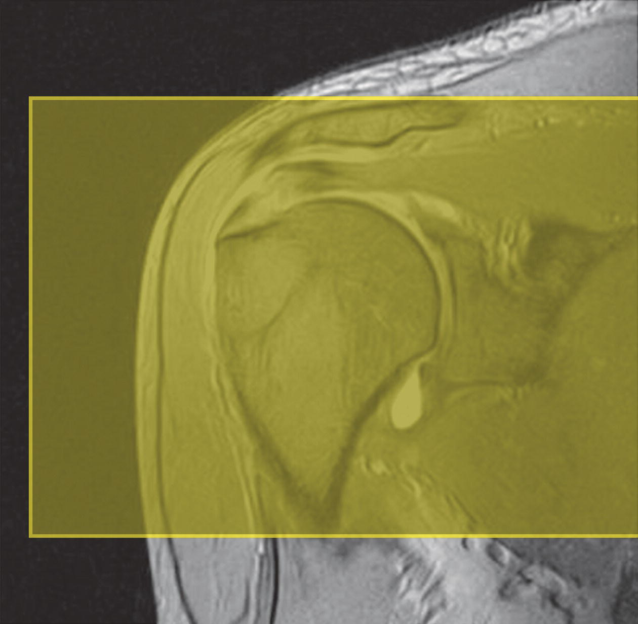
Coronal/oblique SE/FSE T1 (Figure 13.4)
Coronal/oblique SE/FSE T2 +/− tissue suppression (Figures 13.7 and 13.8)
Axial SE/FSE/oblique T1+ tissue suppression
Additional sequences
Sagittal/oblique SE/FSE T1
Sagittal/oblique/axial FSE PD/T2 +/– tissue suppression
3D FSE with variable refocused flip angle PD or T2 contrast +/– tissue suppression
3D GRE T2* BGE/GRE
MR arthrography (Figures 13.10 and 13.11)
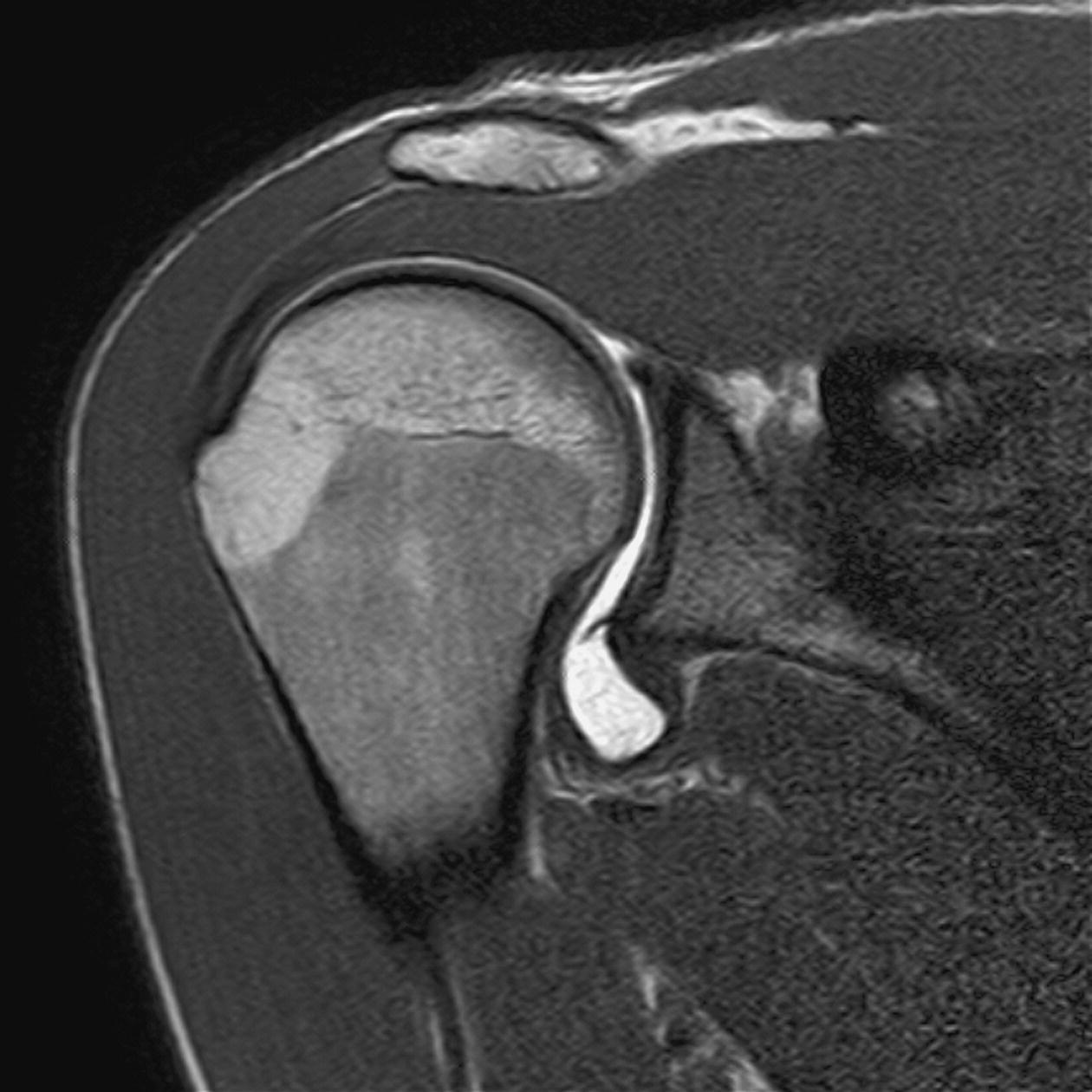
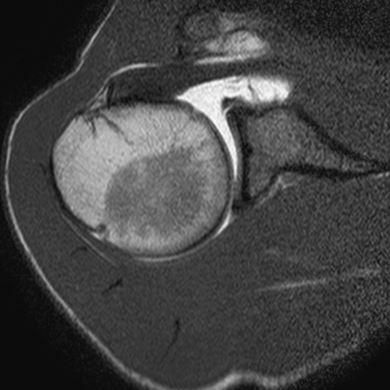
Image optimization
Technical issues
Artefact problems
Patient considerations
Contrast usage
Related posts:

Stay updated, free articles. Join our Telegram channel

Full access? Get Clinical Tree


