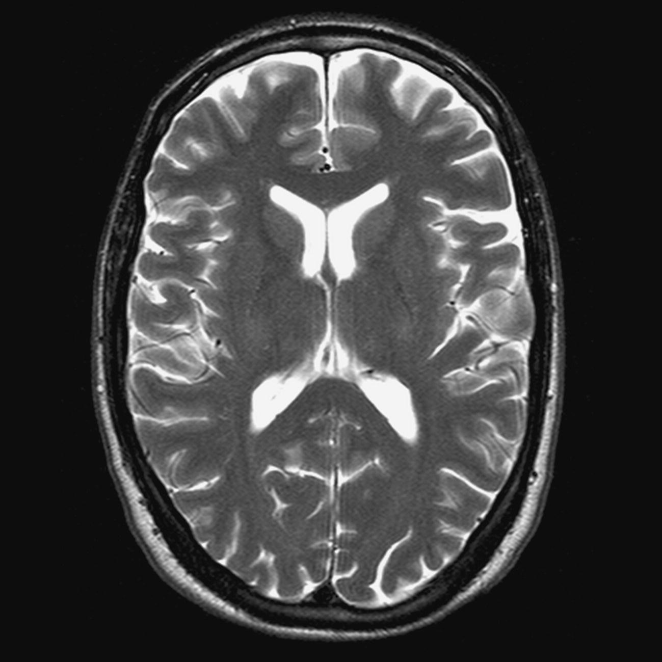
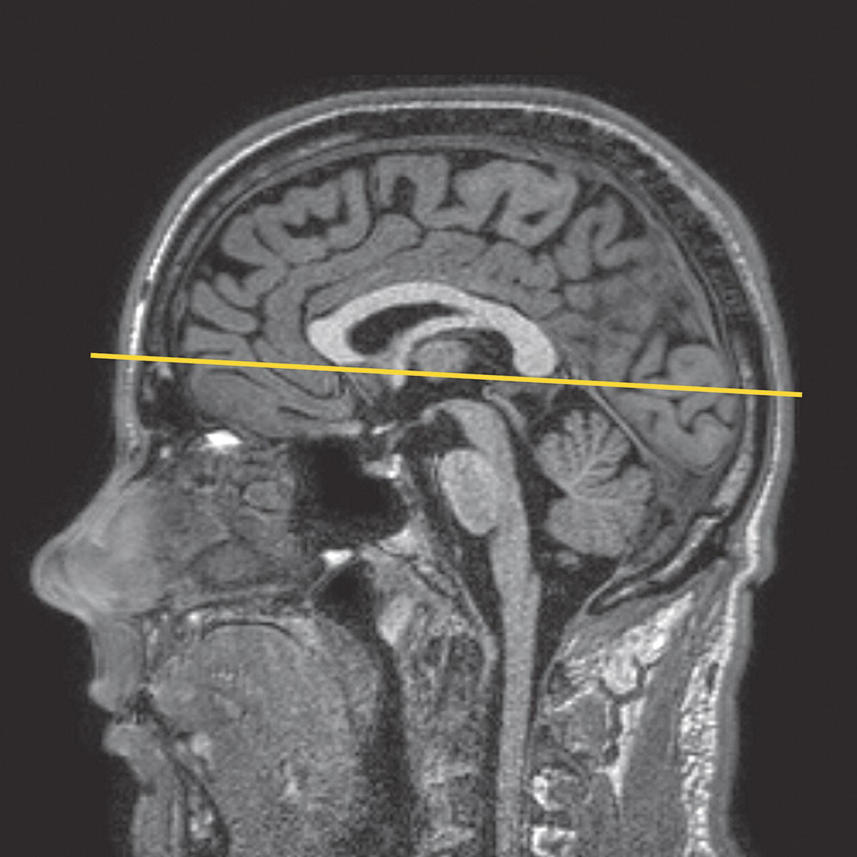
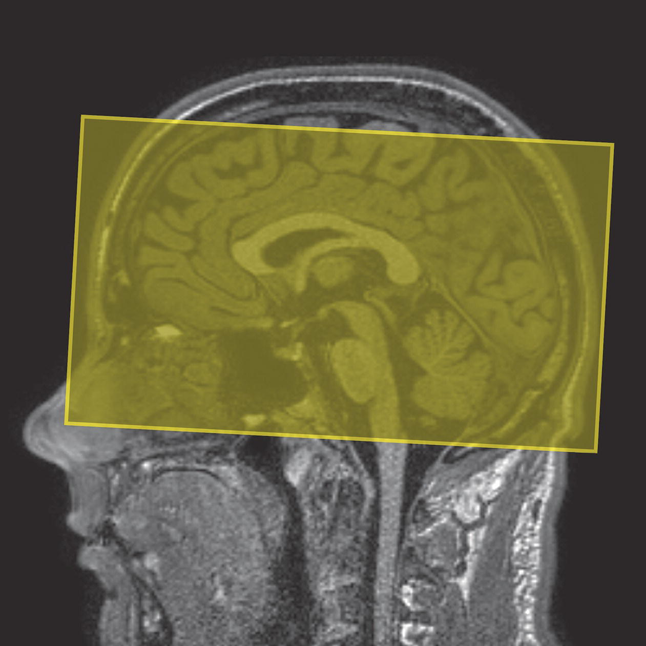
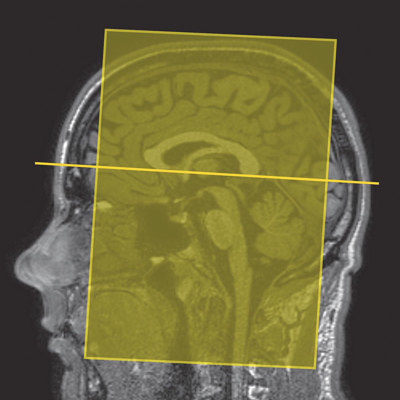
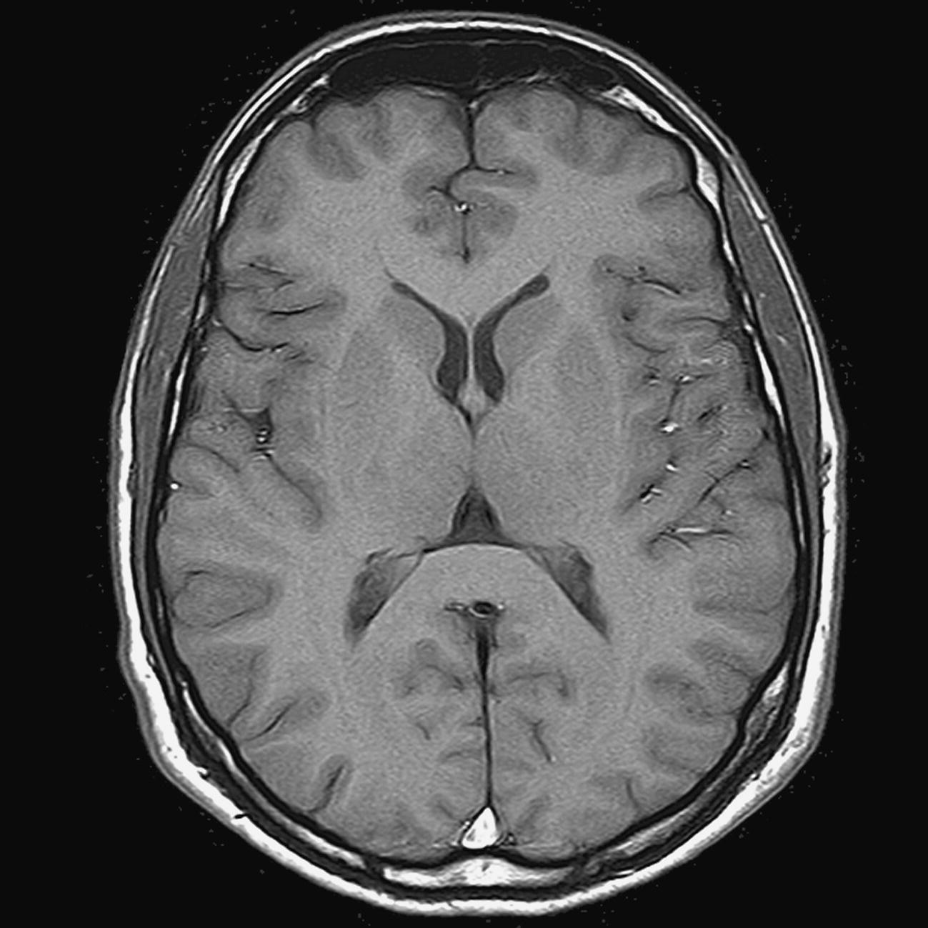
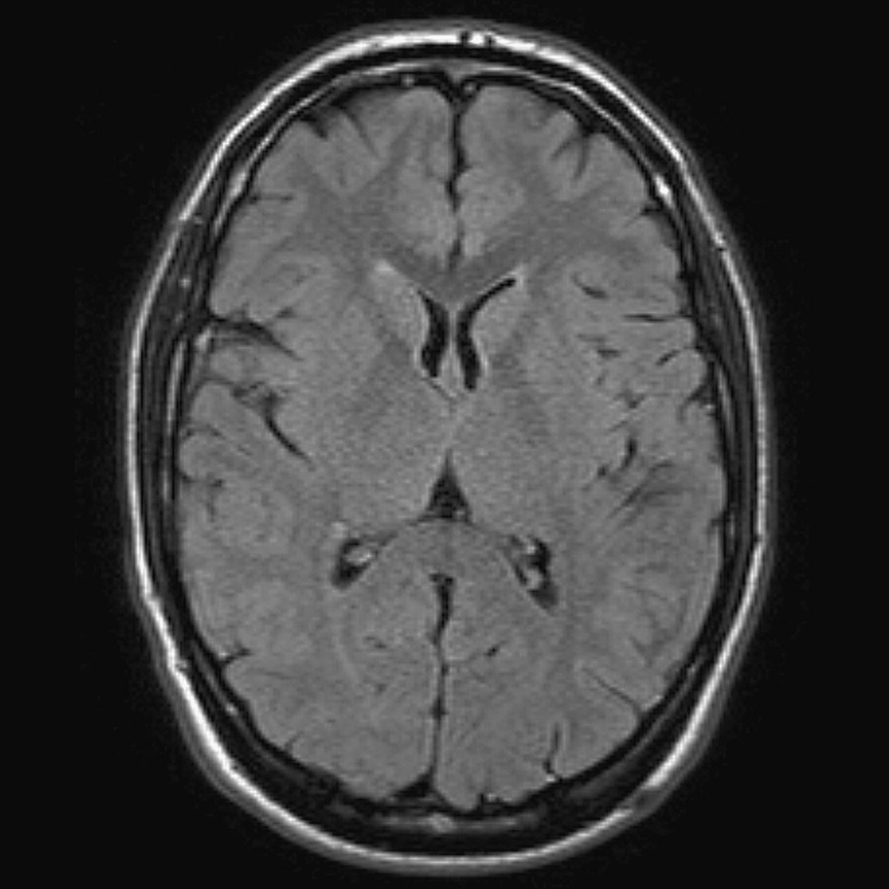
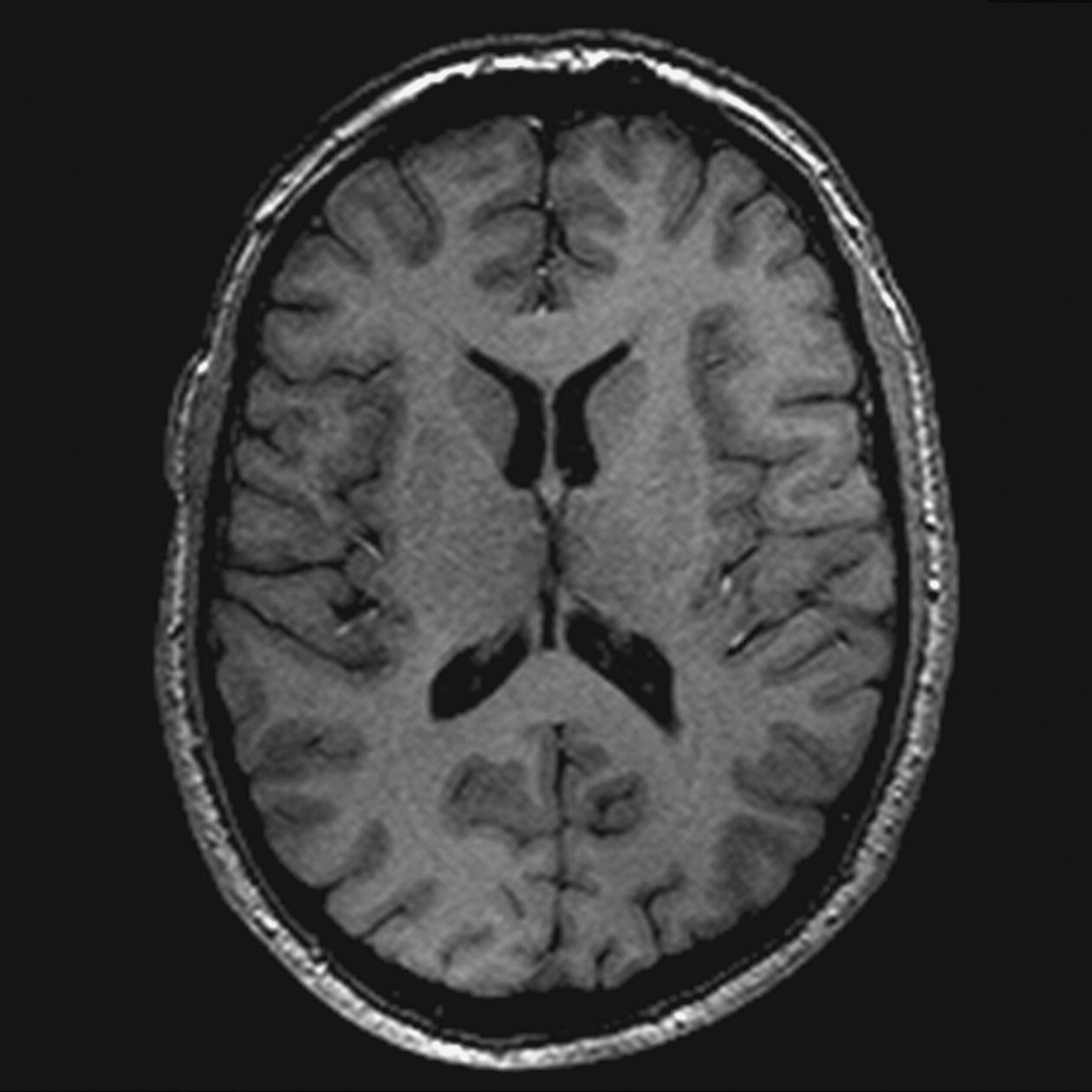
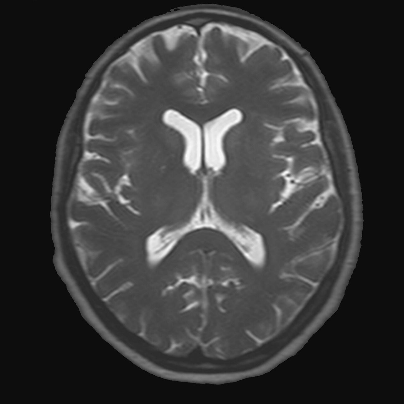
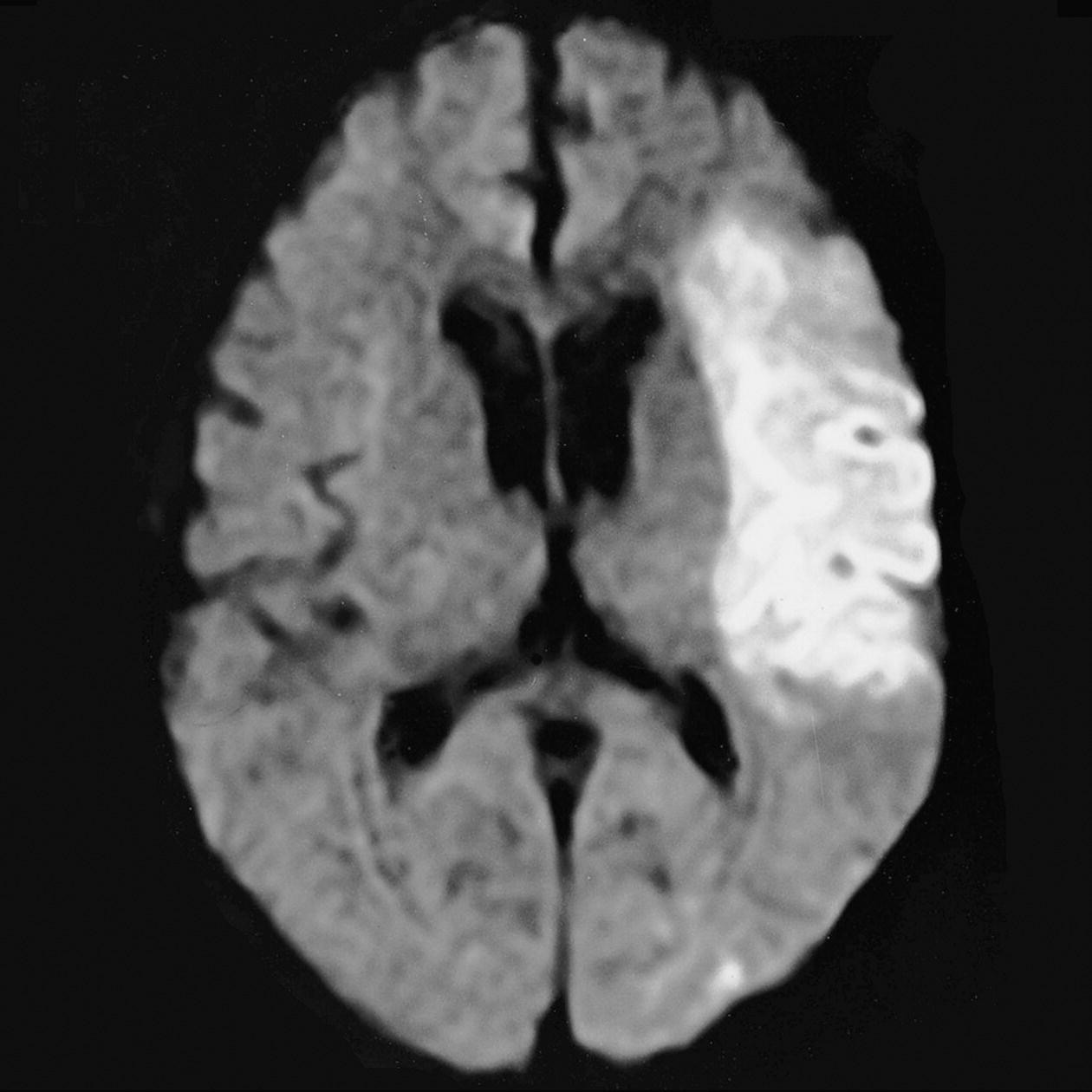
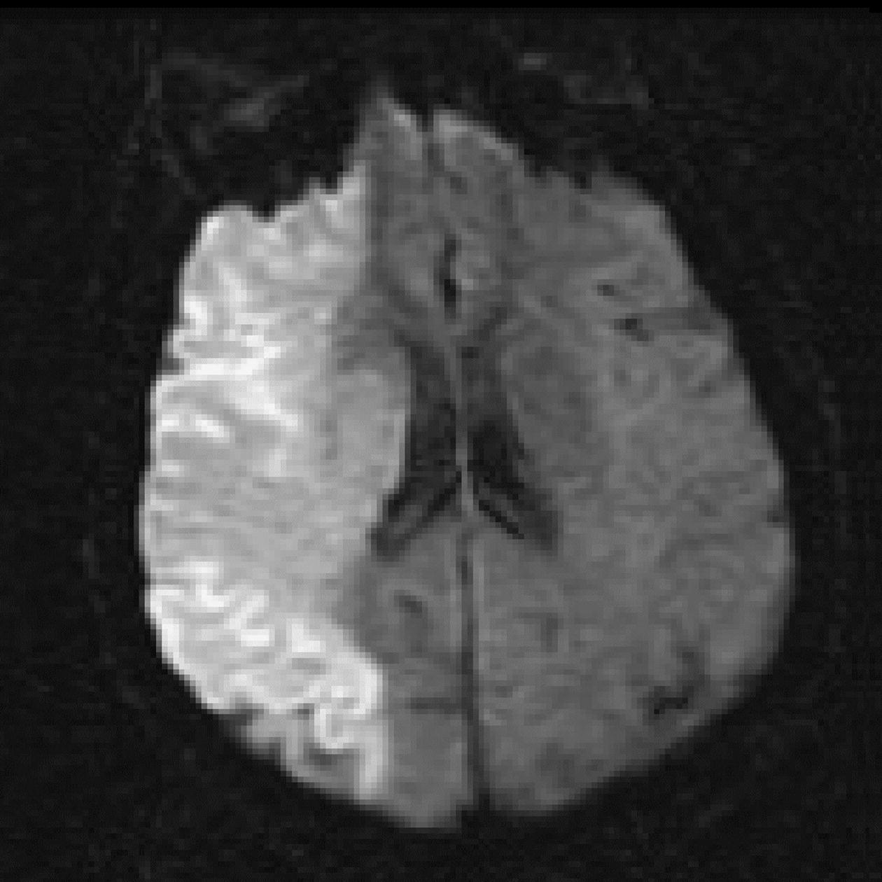
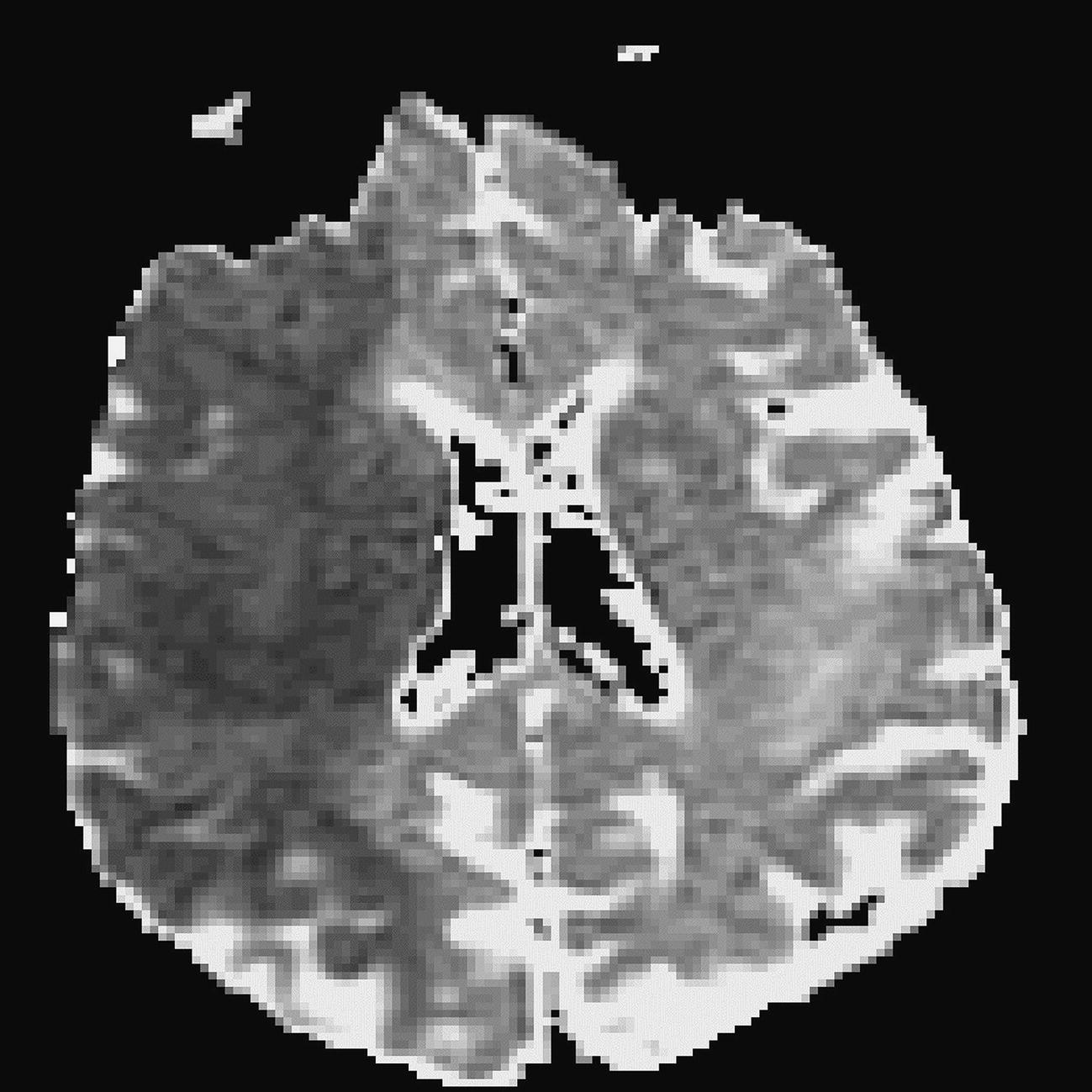
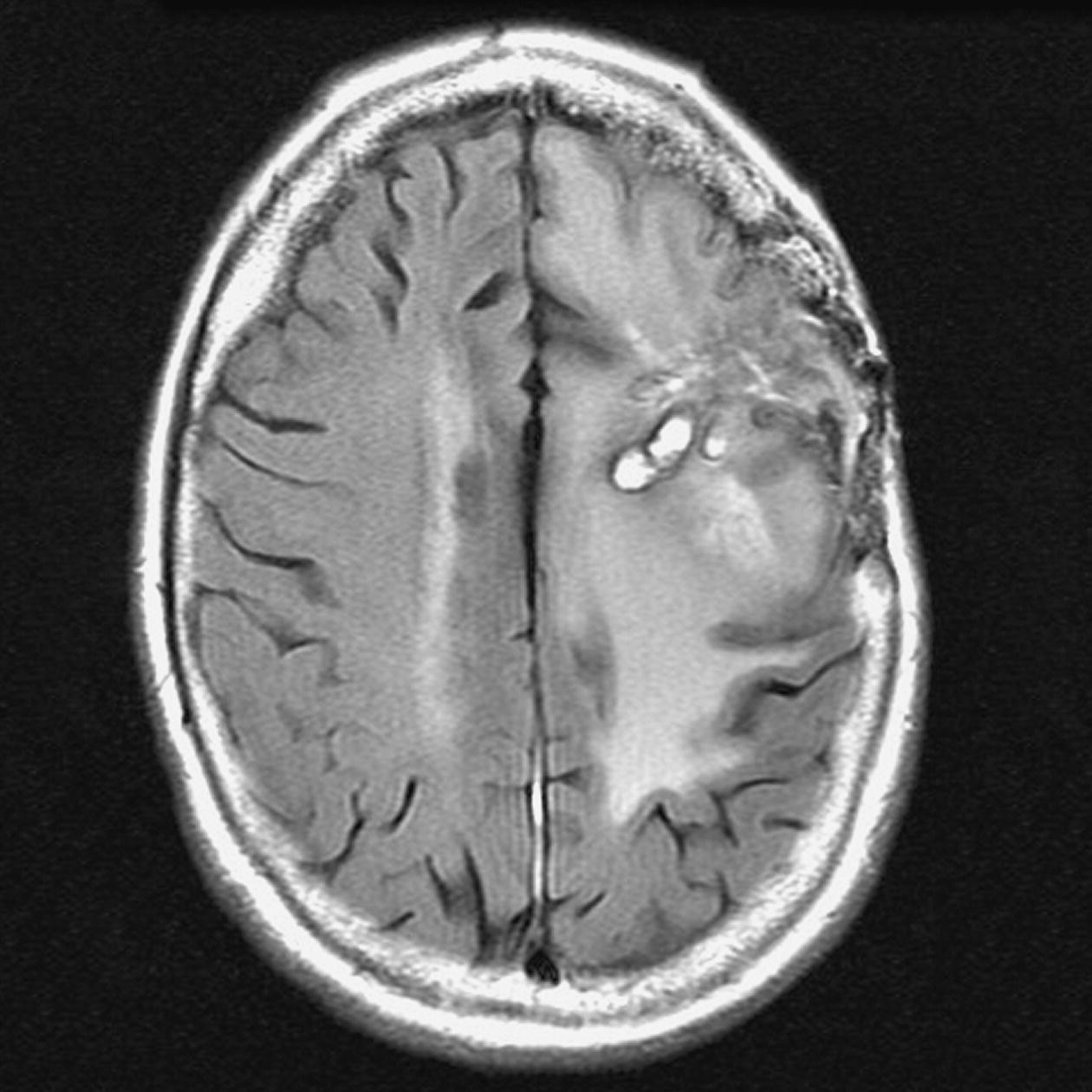
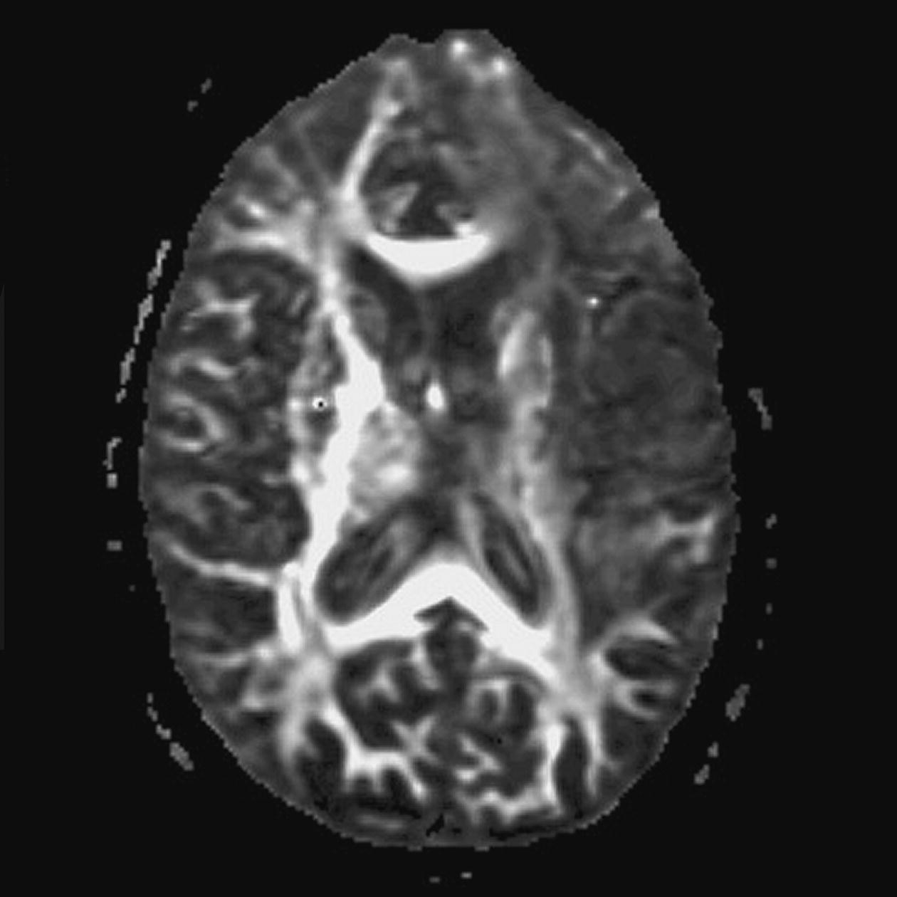
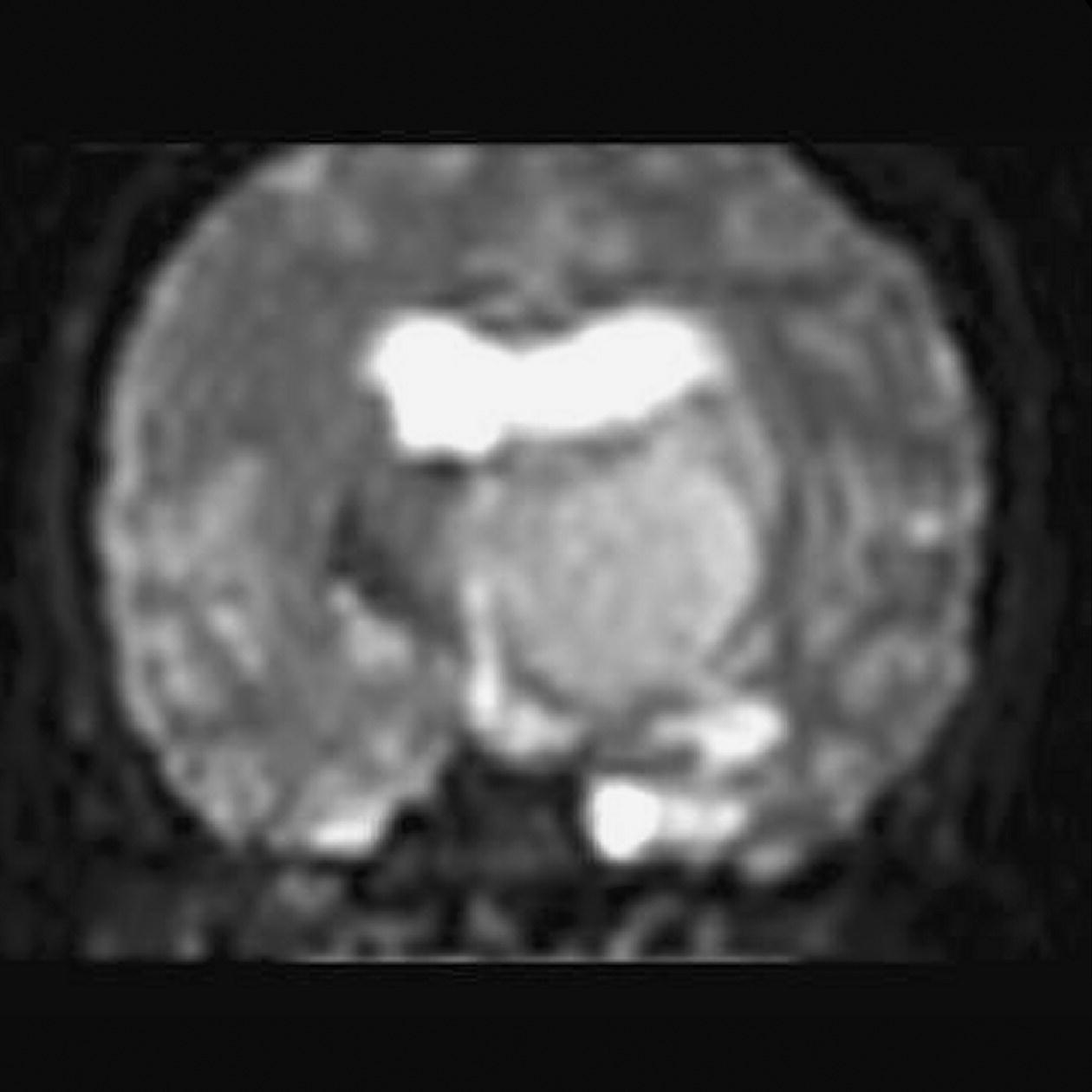
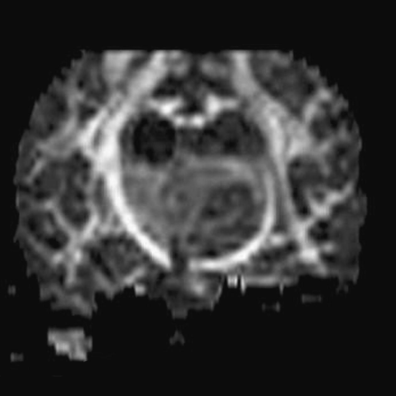
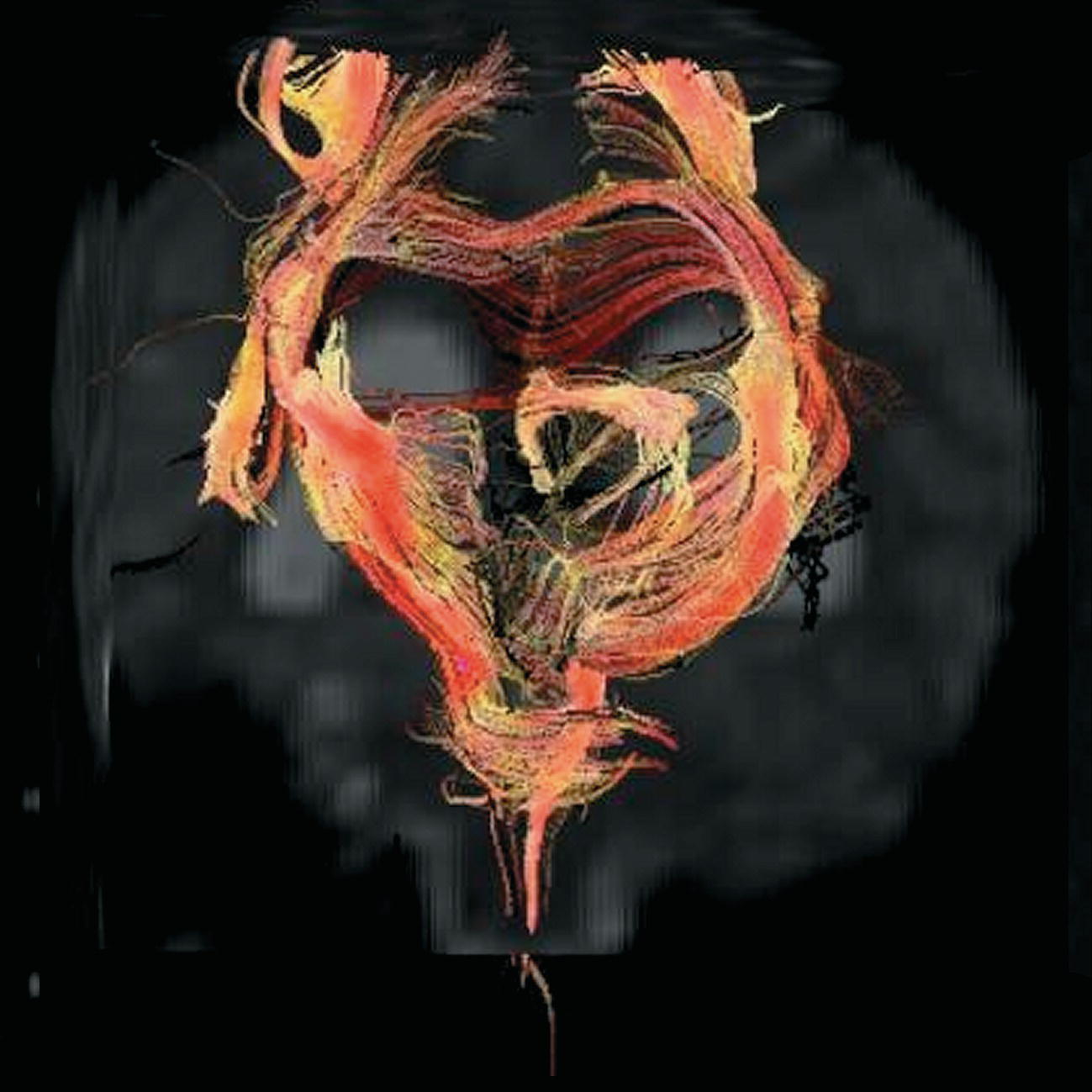
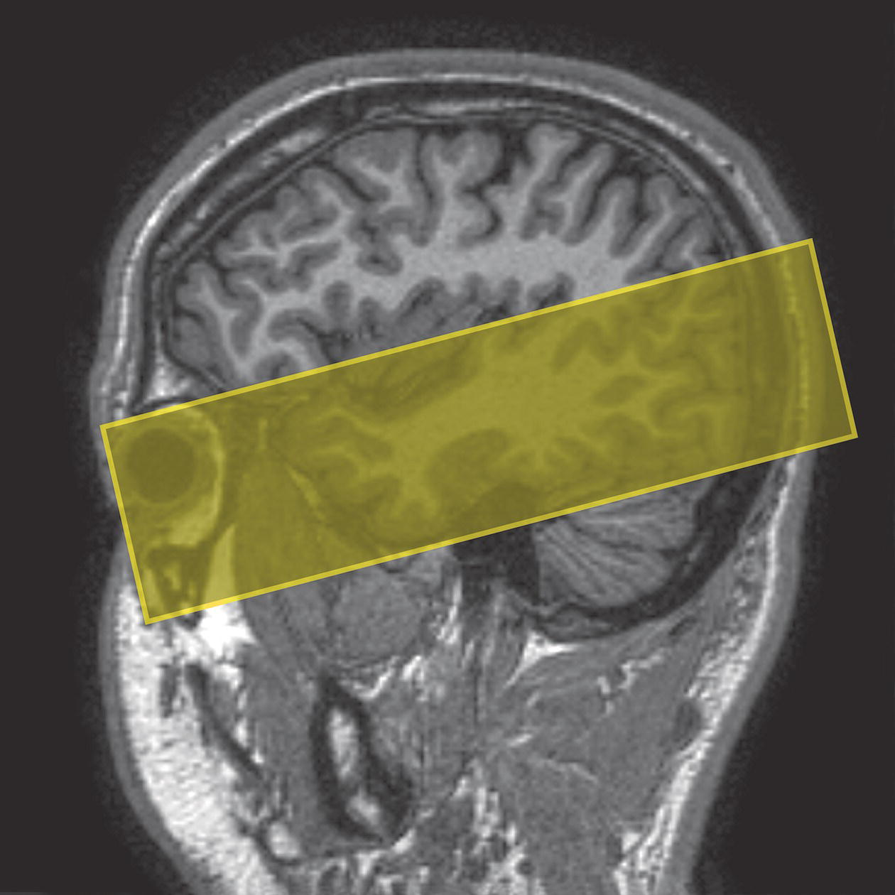
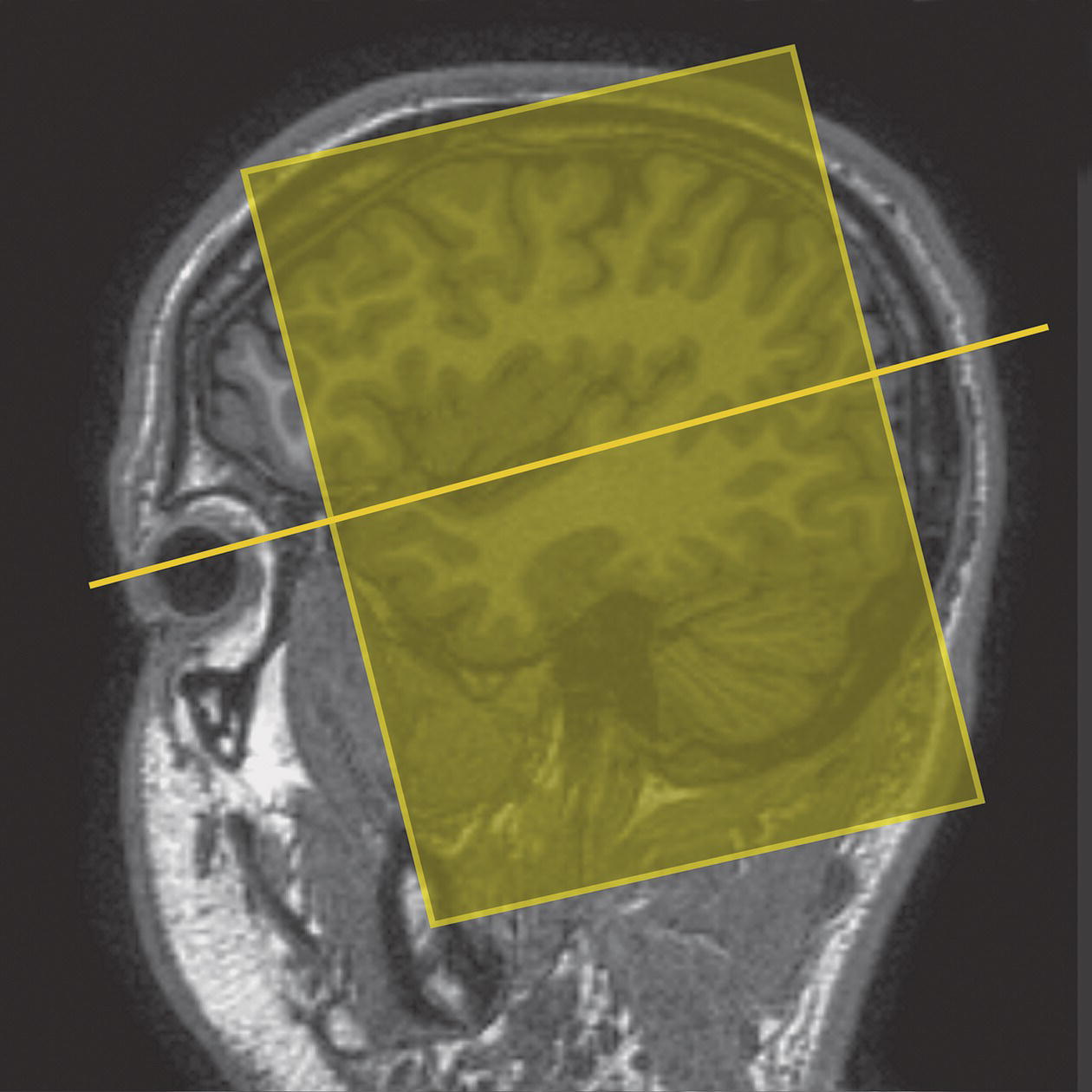
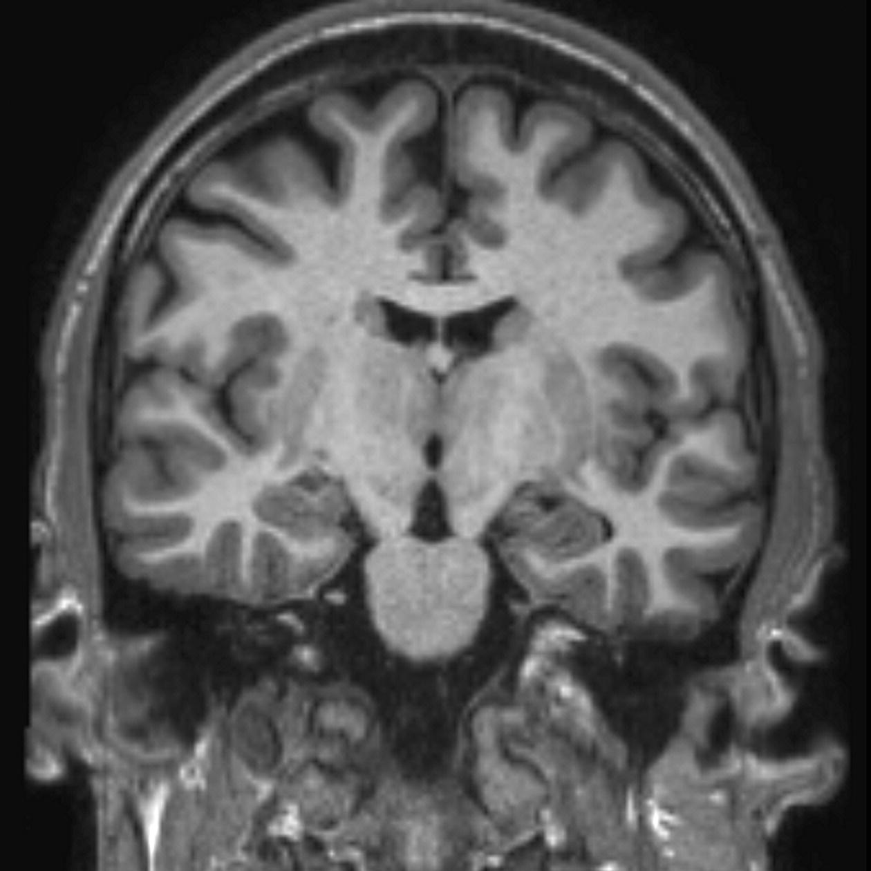
8 Table 8.1 Summary of parameters The figures given are for 1.5 T and 3 T systems. Parameters are dependent on field strength and may need adjustment for very low or very high field systems. Figure 8.1 Transverse aspect of the brain showing inferior structures. Figure 8.2 Oblique aspect of the brain showing inferior structures. The patient lies supine on the examination couch with their head within the head coil. The head is adjusted so that the inter-pupillary line is parallel to the couch and the head is straight. The patient is positioned so that the longitudinal alignment light lies in the midline, and the horizontal alignment light passes through the nasion. Straps and foam pads are used for immobilization. Medium slices/gaps are prescribed on each side of the longitudinal alignment light from one temporal lobe to the other. The area from below the foramen magnum to the top of the head is included in the image. L 37 mm to R 37 mm Figure 8.3 Axial/oblique FSE T2-weighted image of the brain showing normal appearances. Medium slices/gaps are prescribed from below the foramen magnum to the superior surface of the brain. Slices may be angled so that they are parallel to the anterior–posterior commissure axis. This enables precise localization of lesions from reference to anatomy atlases (Figures 8.4 and 8.5). Many sites have replaced the PD sequence with T2-FLAIR. T2-FLAIR sequences can be helpful when acquired following the injection of a contrast agent. Due to the T1 contribution of inversion sequences, ‘enhancing’ lesions and structures are hyper-intense. This aids the visualization of leptomeningeal metastasis and/or meningitis. The only caveat is that ‘enhancement’ of meningiomas is not seen on post-contrast T2-FLAIR due to their short T2 relaxation times. SS-FSE or SS-EPI may be a necessary alternative for a rapid examination in uncooperative patients. Figure 8.4 Sagittal SE T1-weighted midline slice of the brain showing the axis of the anterior and posterior commissures. Figure 8.5 Sagittal SE T1-weighted midline slice of the brain showing slice prescription boundaries and orientation for axial/oblique imaging. As for axial PD/T2, except prescribe slices from the cerebellum to the frontal lobe (Figure 8.6). Figure 8.6 Sagittal SE T1-weighted image showing slice prescription boundaries and orientation for coronal imaging. Figure 8.7 Axial IR T1-weighted image using a TI of 700 ms. Slice prescription as for axial/oblique T2. This sequence is especially useful in imaging the paediatric brain. White matter does not fully myelinate until approximately five years of age; therefore, in very young patients, grey matter and white matter have very similar T1 relaxation times, and the CNR between these tissues is small on SE T1 sequences. Figure 8.8 Axial/oblique FLAIR image of the brain. Periventricular abnormalities will have a high signal intensity in contrast to the low signal of CSF which has been nulled using a long TI. Slice prescription as for axial/oblique T2. This sequence provides a rapid acquisition with suppression of CSF signal. It may be useful when examining periventricular or cord lesions such as MS plaques. Figure 8.9 Axial/oblique incoherent (spoiled) GRE image of the brain. Slice prescription as for axial/oblique T2. Pre- and post-contrast scans are common especially for tumour assessment. Figure 8.10 SS-FSE T2-weighted image of the brain. The entire brain was scanned in 40 s. Useful for rapid imaging in uncooperative patients. This sequence is useful for high-resolution imaging of small structures within the brain. If reformatting of slices is desired, an isotropic data set must be acquired (see Volume imaging under Parameters and trade-offs in Part 1). Additionally, due to the short TE utilized with the spoiled GRE sequence, flow artefacts are essentially eliminated. Figure 8.11 SS-EPI image of the brain. The entire brain was scanned in 14 s. Due to sensitivity to magnetic susceptibilities, these sequences demonstrate haemorrhage better than SE and FSE. Slice prescription as for axial/oblique T2. MT is a useful sequence to improve visualization of lesions such as metastasis, and some low-grade tumours, as grey and white matter loses 30–40% of its signal when a MT pulse sequence is utilized. The CNR between lesions and the surrounding brain is therefore increased (see Pulse sequences in Part 1). Figure 8.12 DWI showing large area of high signal on right. High signal on a DWI can be the result of restricted diffusion or ‘T2 shine-through’. Figure 8.13 Calculated ADC image showing restricted diffusion (acute stroke) as low signal. Small area of high signal in right posterior represents ‘T2 shine-through’. Slice prescription as for axial/oblique T2. This sequence is important in the investigation of early stroke. It is also utilized in paediatric patients to investigate the effects of hypoxia and myelination patterns. A b-value of 800–1000 s/mm2 is selected (the higher the b-value, the more diffusion weighting). Isotropic diffusion should be acquired (i.e. diffusion gradients applied in all three axes) (see Pulse sequences in Part 1). A DWI sequence is most often acquired using a T2-weighted EPI sequence. In a standard T2-weighted EPI sequence, there is not enough motion (diffusion) of the extracellular water during the imaging cycle to result in dephasing of the water protons. Diffusion gradients are therefore utilized to increase the sensitivity to the motion of the extracellular water molecules. The b-value controls the amplitude, duration and/or timing of these diffusion gradients and thus determines the amount of diffusion weighting in a diffusion sequence. Increasing the b-value increases the sensitivity to the motion (diffusion) of extracellular water in tissue and thus increases the diffusion weighting. The signal in areas of normal diffusion is reduced due to the dephasing of the water protons in the presence of these diffusion gradients. The more restricted the diffusion, the less dephasing of the water protons and higher signal will be seen on the diffusion image. On most MR systems, both the b = 0 image (i.e. the T2-weighted EPI image) and the diffusion image with the b value chosen by the operator will be displayed. Some systems may also display three additional images per slice location. These are the images obtained during the diffusion acquisition. The diffusion gradients are applied in each of the three orthogonal planes (X, Y and Z) measuring the diffusion in each of those directions. The data are then averaged to produce the final ‘trace’ or diffusion-weighted image displayed. It is important to remember that high signal seen on a diffusion-weighted image may actually be high signal from spins with a long T2 relaxation time ‘shining through’. These so-called ‘T2 shine-through’ effects are eliminated by the calculation and production of an apparent diffusion coefficient (ADC) map or image. The ADC expresses the amount of motion of extracellular water. The ADC image is calculated from the b-value of 0 and the b-value used in the diffusion acquisition (most commonly 1000 mm/s2 in a DWI exam of the brain) to produce a ‘2-point’ ADC image (Figure 8.13). In some situations, one may acquire a DWI with two b-values. That, along with the b-value of 0, would be used to calculate a ‘3-point’ ADC image. In any event, the pixel values in an ADC image represent the ADC of pixels in the image. In areas with restricted diffusion (i.e. low ADC), the pixel values are dark. A high ADC, seen in the presence of mobile water protons will result in a bright pixel on the ADC image. Calculating and producing an ADC image is very important in distinguishing between acute and chronic stokes. Depending on the MR system, the ADC image may be produced automatically or it may require some minor additional processing steps. When the diffusion of water along the three orthogonal directions of the magnet (X, Y and Z) is measured and the average obtained, only isotropic diffusion information is acquired, that is, diffusion that is random in direction. In the brain, this is seen in grey matter. In white matter, the structure of the tissue ‘orders’ the diffusion. In white matter, diffusion is ordered along the white matter tracts. This type of ordered diffusion is referred to as anisotropy (anisotropic diffusion). In order to image anisotropic diffusion, diffusion in more than three axes is measured. In physics, a tensor is basically motion as a function of direction. DTI is essentially imaging diffusion that is ordered in direction (anisotropic rather than isotropic). At a minimum, DTI must measure the diffusion along at least six axes. In clinical practice, 12 or more directions are measured. Due to a loss in SNR as the number of directions measured increases, DTI is particularly useful at high field strengths such as 3 T. DTI is currently used for mapping white matter tracts as fractional anisotropy (FA) maps, or as tractography images (Figures 8.14, 8.15, 8.16, 8.17 and 8.18). Figure 8.14 T2-weighed FLAIR showing lesion. Figure 8.15 Fractional anisotropy (FA) map showing anisotropic (ordered) diffusion in the white matter tracts. Figure 8.16 Coronal T2-weighted EPI demonstrates lesion. Figure 8.17 FA map shows white matter tracts relative to the lesion. Figure 8.18 Tractography demonstrates tract orientation relative to the lesion. Slice prescription as for axial/oblique T2. This sequence provides temporal resolution of enhancing lesions and indicates activity. Injection of a gadolinium bolus should begin immediately after the scan is initiated. Post-enhancement T1 imaging follows the perfusion series (see Pulse sequences and its subheading Dynamic imaging in Part 1). The use of an MR-compatible contrast injector greatly increases the consistency of perfusion information. Furthermore, in order to optimize the susceptibility effects, a rapid bolus of contrast is necessary. A minimum injection rate of 4 ml/s is preferable. The amount or volume injected may vary depending on concentration of the contrast media, relaxivity of the contrast media, field strength, and/or pulse sequence utilized. At 1.5 T, the strongest effects are seen using a GRE-EPI sequence. If such a sequence is used, 0.1 mmol/kg is typically adequate. Due to the increased susceptibility effects seen with a GRE-EPI sequence, only information regarding large vessel perfusion is obtained. If one wishes to obtain information relating to small vessel perfusion, then a SE-EPI sequence should be utilized. It is important to remember however that due to the reduced susceptibility effects obtained with the SE-EPI sequence, a higher dose or concentration of gadolinium may be necessary. Not all gadolinium agents have the same effect on T1 and T2 relaxation times. There are some agents with higher relaxivities. These agents, when used for perfusion imaging, result in greater signal reduction when compared with the same dose of a standard contrast agent due to the increased relaxivity. At 3.0 T, susceptibility effects are increased as a function of the field strength and allow for either a reduced dose of gadolinium (0.5 mmol/kg) with a GRE-EPI sequence or a standard dose (0.1 mmol/kg) of gadolinium with a SE-EPI sequence. SE-EPI sequences also result in fewer susceptibility artefacts. In summary, the amount of gadolinium used for perfusion imaging is dependent upon the type of contrast agent used, field strength and acquisition technique selected. When perfusion imaging is utilized for stroke imaging, the area affected by the stroke appears as either an area of late arriving contrast or totally non-perfusing. When imaging a tumour, however, the area of abnormal perfusion will often be demonstrated as an area of hyper-perfusion. The images in Figures 8.19 and 8.20 illustrate this effect. The area of residual tumour is indistinguishable from the adjacent tissue due to oedema and other changes. The perfusion data clearly show an area of increased or hyper-perfusion indicating residual or recurrent tumour. Figure 8.19 T2-weighted image shows large area of oedema following treatment. Figure 8.20 Perfusion data shows area of hyper-perfusion within the oedema indicating recurrent tumour. Using a quadrature or multi-coil array yields high and uniform signal. Using a multi-coil array with greater than four channels however may require the use of a uniformity correction algorithm to produce an image with uniform signal throughout. Regardless of the coil selected, images with excellent SNR and spatial resolution should be easily attainable in reasonable scan times. FSE is the pulse sequence most often utilized for acquiring PD- and T2-weighted images due to its shorter scan times compared with CSE. There is some debate as to whether PD- and T2-weighted images should be acquired as part of a dual echo acquisition or separately. TRs in the order of 3500 ms or higher are usually employed in T2-weighted FSE imaging. For PD-weighted images of the brain, however, such a high TR is not optimal. If the TR is increased above 2000 ms, signal intensity of CSF increases due to reduced saturation and the high proton density of CSF. This may reduce contrast between some periventricular lesions such as MS and CSF. This a major reason why T2-FLAIR sequences are now generally preferred over PD-weighted sequences in the brain. Blurring may be more prominent with the long ETL traditionally associated with T2-weighted FSE. A short ETL and TE are required for PD weighting to minimize T2 effects, whereas a long ETL and TE are required for T2 contrast. Blurring increases the longer the train of echoes goes out in time. Due to T2 dephasing, the echoes that occur a long way out in the train have lower signal amplitude than those at the beginning of the train. If the effective TE does not coincide with these late echoes, data from them are mapped into the resolution lines of k-space and result in blurring. The echo spacing is also important as if the echo spacing is long, the final echoes in the train will occur much later and therefore be of lower signal intensity than if the spacing is short, even in a train containing a relatively small number of echoes. Conversely, if the echo spacing is short, the final echoes are collected earlier and will be of higher signal intensity, even in a train containing a larger number of echoes. (Note: The term ‘echo train length’ refers to the number of echoes collected rather than the time taken to do so.) The exact method of controlling the echo spacing varies between manufacturers. Faster switching gradients (i.e. higher slew rates) allow for a long ETL with tight echo spacing. Generally speaking, the echo spacing should be kept as low as possible to minimize blurring (typically between 10 and 15 ms). As a result of these limitations, some advocate acquiring the PD- and T2-weighted images separately as this permits the use of a shorter TR and ETL in the PD acquisition. Alternatively, some manufacturers allow the echo train to be split in dual echo FSE acquisitions so that the PD-weighted image is acquired from the first echoes in the train and the T2-weighted image from the later echoes in the train. This results in more optimal weighting for both images but note that in FSE, unlike CSE, the acquisition time for PD images is shorter than that for T2 or dual echo. This is because a TR of 2000 ms is used rather than 10,000 ms. There is therefore a time-saving to be made when only PD weighting is required. In CSE, in the interests of reducing scan time, T2-weighted images already have a relatively short TR. PD- and T2-weighted images therefore have similar acquisition times and are routinely acquired simultaneously in a dual echo sequence. There is therefore no time-saving to be made by acquiring PD-weighted images on their own. Despite the time advantages of using FSE in the brain, the multiple 180° pulses in an FSE sequence reduce the sensitivity to haemorrhagic lesions. If haemorrhagic lesions are suspected, a coherent GRE sequence may be acquired in addition to the regular sequences (TEs of 15–25 ms). It should also be noted that in many centres, T2-FLAIR images have replaced PD-weighted images in the brain. T2-FLAIR sequences typically demonstrate subarachnoid blood very well. Due to the relatively high SNR, only a few NEX/NSA are usually required to achieve adequate image quality. However, this may not be the case when examining small structures with thin slices and/or a smaller FOV. In such a situation, it may be necessary to increase the NEX/NSA. The receive bandwidth may be decreased to increase the SNR without significantly increasing chemical shift artefact. However, generally speaking, as the receive bandwidth is reduced, the echo spacing increases and could result in an increase in FSE blurring. Rectangular FOV or parallel imaging may be utilized to reduce scan times in axial and/or coronal imaging with the phase encoding direction being R to L. The main source of artefact in the brain is from flow motion of the carotid and vertebral arteries. A spatial pre-saturation pulse placed I to the FOV reduces this significantly. In large FOV imaging, there is no need to place spatial pre-saturation pulses anywhere other than I, as there is no flow coming into the FOV from any other direction. If a small FOV is used, S or R and L spatial pre-saturation pulses are sometimes necessary. GMN also minimizes artefact especially in the posterior fossa. However, it not only increases the signal in vessels but also the minimum TE available and is therefore usually reserved for T2- and T2*-weighted sequences. Pe gating minimizes artefact even further, but as the scan time is dependent on the patient’s heart rate, it is rather time-consuming and is not therefore commonly used. Ghosting occurs along the phase encoding axis, which may be swapped in order to remove the artefact away from the ROI. However, in most examinations of the brain, this strategy is unnecessary as flow suppression techniques are satisfactory. Uncooperative patients are likely to cause motion artefacts unless very rapid sequences are employed. FSE, while faster than SE, often produces more severe motion artefacts because one of the central lines of k-space is being filled during each TR period. SS-FSE techniques greatly reduce the effects of motion and allow the whole brain to be examined in approximately 30 s by using an ETL as high as 128. SS-FSE sequences, although very rapid, may still show some degree of patient motion. In order to eliminate the effect of patient motion completely, SS-EPI techniques should be used. However, EPI sequences are prone to air/tissue magnetic susceptibility artefact (see Pulse sequences in Part 1). Newer acquisition techniques, which fill k-space in a different fashion, can also be employed to reduce or even eliminate the effects of patient motion. These techniques are known as PROPELLER, BLADE, MultiVane and JET (depending on the manufacturer). Off-resonance effects (mainly magnetic susceptibility) contribute greatly to the distortion artefacts commonly seen on SS-EPI sequences used to acquire DWI images. These artefacts increase with higher field strength systems (such as 3 T) but can be reduced by decreasing the number of phase encoding views (e.g. rectangular FOV or parallel imaging techniques). Unfortunately, if one simply reduces the phase matrix, this results in a reduction in spatial resolution. Claustrophobia is often troublesome because of the enclosing nature of the head coil. In addition, neurological factors may increase the likelihood of patient movement. Examples of these are epilepsy, Parkinson’s disease and reduced awareness or consciousness. Reassurance, and in extreme circumstances sedation or general anaesthesia, is sometimes required. Due to excessively loud gradient noise associated with some sequences, earplugs or headphones must always be provided to prevent hearing impairment. EPI sequences employ very rapid gradient rise times. The faster the rise times, the greater the chance for inducing peripheral nerve stimulation. To reduce this probability, the frequency encoding direction should be R to L for all axial EPI sequences in the brain. This is not necessary with SS-FSE sequences. Additionally, patients should be instructed to place their arms by their sides and to not cross their ankles to prevent creating a loop that could precipitate excessive induction of current. Contrast agents have several uses in standard brain imaging. They are usually required for tumour assessment, inflammatory processes such as MS or the evaluation of vascular abnormalities. Infectious processes, such as abscesses, are very susceptible to enhancement. In addition, the meninges enhance so that infectious tuberculosis, leptomeningeal tumour spread and post-trauma meningeal irritation can be visualized. Contrast is also used to ascertain the age of an infarct. Very recent infarcts may enhance to some degree, but maximum response to contrast usually occurs after the blood–brain barrier has been breached. Old or chronic infarcts do not enhance. Either SE or incoherent (spoiled) GRE T1 is the sequence of choice after contrast. If a 3D incoherent (spoiled) GRE sequence is acquired using isotropic voxels, the data set may be reformatted in other planes and/or slice locations. Perfusion imaging, with a rapidly infused bolus of gadolinium, is useful for measuring the activity of a lesion. In these cases, rapid acquisitions such as SS-FSE or EPI are required. Figure 8.21 The temporal lobe and its relationships. The patient lies supine on the examination couch with their head within the head coil. The head is adjusted so that the inter-pupillary line is parallel to the couch and the head is straight. The patient is positioned so that the longitudinal alignment light lies in the midline, and the horizontal alignment light passes through the nasion. Straps and foam pads are used for immobilization. Medium slices/gaps are prescribed on either side of the longitudinal alignment light through the whole head. The area from the foramen magnum to the top of the head is included in the image. L 37 mm to R 37 mm Thin slices/gap or interleaved slices are angled parallel to the temporal lobe that can be seen on a lateral slice on the sagittal images (Figure 8.22). Prescribe the slices from the inferior aspect of the temporal lobes to the superior border of the body of the corpus callosum. Figure 8.22 Sagittal SE T1-weighted image through a temporal lobe showing slice prescriptions boundaries and orientation for axial/oblique imaging of the temporal lobes. As for the axial/oblique T2, except thin slices interleaved are angled perpendicular to the axials (Figure 8.23). Figure 8.23 Sagittal SE T1-weighted image through a temporal lobe showing slice prescription boundaries and orientation for coronal/oblique imaging of the temporal lobes. Slices are prescribed from the posterior portion of the cerebellum to the anterior border of the genu of the corpus callosum. Figure 8.24 Coronal incoherent (spoiled) T1-weighted GRE image through the hippocampi acquired as part of a 3D acquisition. Thin slices are either prescribed through the temporal lobes only (medium number of slice locations), or the whole head (large number of slice locations). For hippocampal measurements, slices are prescribed from the posterior portion of the cerebellum to the anterior border of the genu of the corpus callosum. Hippocampal volumes are measured by using system software to calculate the area of the hippocampus on each slice and multiplying this by the depth of the slice slab. If reformatting of slices is desired, then an isotropic data set should be acquired (see Volume imaging under Parameters and trade-offs in Part 1). Figure 8.25 Coronal IR-FSE T2-weighted image with a TI selected to null the signal from the white matter (300 ms). Figure 8.26 Coronal IR-FSE T2-weighted image video inverted to better demonstrate white matter lesions. Slice prescription as for axial/oblique/coronal/oblique FSE T2. This sequence often provides images with high contrast between grey matter and white matter. A TI selected to null the signal from the white matter (about 300 ms) can be used to increase the grey/white (G/W) contrast in the hippocampal region. Images may be video inverted so that the white matter appears white and the grey matter appears grey. This is sometimes useful to increase the conspicuity of white matter lesions, which have a low signal intensity when using this technique and to improve visualization of the basil ganglia. The SNR and contrast characteristics of the temporal lobes are usually excellent as the quadrature head coil and phased array coil yield high and uniform signal. Good spatial resolution is therefore achievable in relatively short scan times. Surface coils placed directly on the patient’s head increase local SNR and resolution, especially in children. However, using this method, other areas of the brain cannot be imaged due to signal fall-off. As lesions within the temporal lobes are often quite small, volume acquisitions are useful as they allow for very thin slices and no gap. As they are mainly utilized to demonstrate anatomy or contrast enhancement, an incoherent (spoiled) GRE that produces PD and T1 contrast is desirable. Alternatively, angling the slices perpendicular to the sylvian fissure in 2D acquisitions often improves visualization of the temporal lobes.
Head and neck
1.5 T
3 T
SE
SE
Short TE
Min–30 ms
Short TE
Min–15 ms
Long TE
70 ms+
Long TE
70 ms+
Short TR
600–800 ms
Short TR
600–900 ms
Long TR
2000 ms+
Long TR
2000 ms+
FSE
FSE
Short TE
Min–20 ms
Short TE
Min–15 ms
Long TE
90 ms+
Long TE
90 ms+
Short TR
400–600 ms
Short TR
600–900 ms
Long TR
4000 ms+
Long TR
4000 ms+
Short TEL
2–6
Short TEL
2–6
Long ETL
16+
Long ETL
16+
IR T1
IR T1
Short TE
Min–20 ms
Short TE
Min–20 ms
Long TR
3000 ms+
Long TR
300 ms+
TI
200–600 ms
TI
Short or null time of tissue
Short ETL
2–6
Short ETL
2–6
STIR
STIR
Long TE
60 ms+
Long TE
60 ms+
Long TR
3000 ms+
Long TR
3000 ms+
Short TI
100–175 ms
Short TI
210 ms
Long ETL
16+
Long ETL
16+
FLAIR
FLAIR
Long TE
80 ms+
Long TE
80 ms+
Long TR
9000 ms+
Long TR
9000 ms + (TR at least 4 × TI)
Long TI
1700–2500 ms (depending on TR)
Long TI
1700–2500 ms (depending on TR)
Long ETL
16+
Long ETL
16+
Coherent GRE
Coherent GRE
Long TE
15 ms+
Long TE
15 ms+
Short TR
<50 ms
Short TR
<50 ms
Flip angle
20–50°
Flip angle
20–50°
Incoherent GRE
Incoherent GRE
Short TE
Minimum
Short TE
Minimum
Short TR
<50 ms
Short TR
<50 ms
Flip angle
20–50°
Flip angle
20–50°
Balanced GRE
Balanced GRE
TE
Minimum
TE
Minimum
TR
Minimum
TR
Minimum
Flip angle
>40°
Flip angle
>40°
SSFP
SSFP
TE
10–15 ms
TE
10–15 ms
TR
<50 ms
TR
<50 ms
Flip angle
20–40°
Flip angle
20–40°
Slice thickness 2D
Slice thickness 3D
Thin
2–4 mm
Thin
<1 mm
Medium
5–6 mm
Thick
>3 mm
Thick
8 mm
FOV
Matrix
Small
<18 cm
Coarse
256 × 128/256 × 192
Medium
18–30 cm
Medium
256 × 256/512 × 256
Large
>30 cm
Fine
512 × 512
Very fine
>1024 × 1024
NEX/NSA
Slice number 3D
Short
1
Small
<32
Medium
2–3
Medium
64
Multiple
>4
Large
>128
PC-MRA 2D and 3D
TOF-MRA 2D
TE
Minimum
TE
Minimum
TR
25–33 ms
TR
28–45 ms
Flip angle
30°
Flip angle
40–60°
VENC venous
20–40 cm/s
VENC venousVENC arterial
60 cm/s
TOF-MRA 3D
TE
Minimum
TR
25–50 ms
Flip angle
20–30°
Brain
Basic anatomy (Figures 8.1 and 8.2)
Common indications
Equipment
Patient positioning
Suggested protocol
Sagittal SE/FSE/incoherent (spoiled) GRE T1
Axial/oblique SE/FSE PD/T2 (Figure 8.3)
Coronal SE/FSE PD/T2
Additional sequences
Axial/oblique IR T1 (Figure 8.7)
Axial/oblique FLAIR/EPI (Figure 8.8)
Axial/oblique SE/FSE/incoherent (spoiled) GRE T1 (Figure 8.9)
SS-FSE T2 (Figure 8.10)
Axial 3D incoherent (spoiled) GRE T1
Axial/oblique GRE/EPI T1/T2 (Figure 8.11)
Axial/oblique SE MT
Axial DWI (Figures 8.12 and 8.13)
Diffusion tensor imaging (DTI)
Axial perfusion imaging
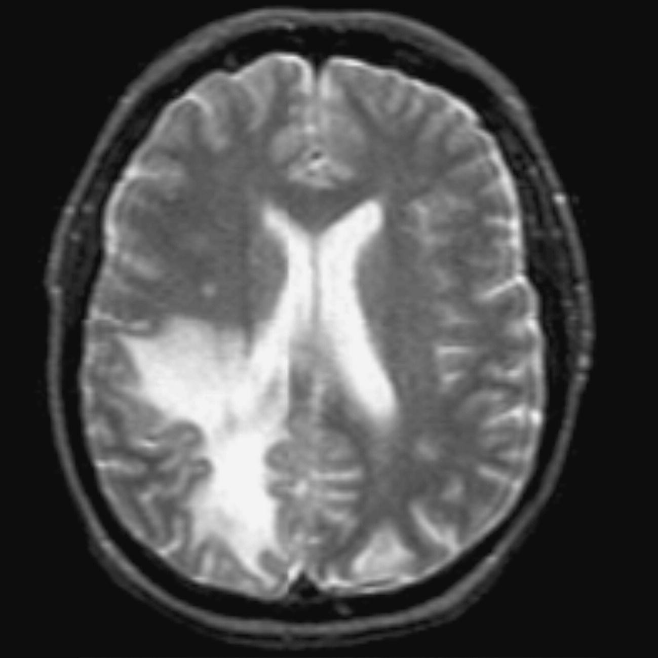
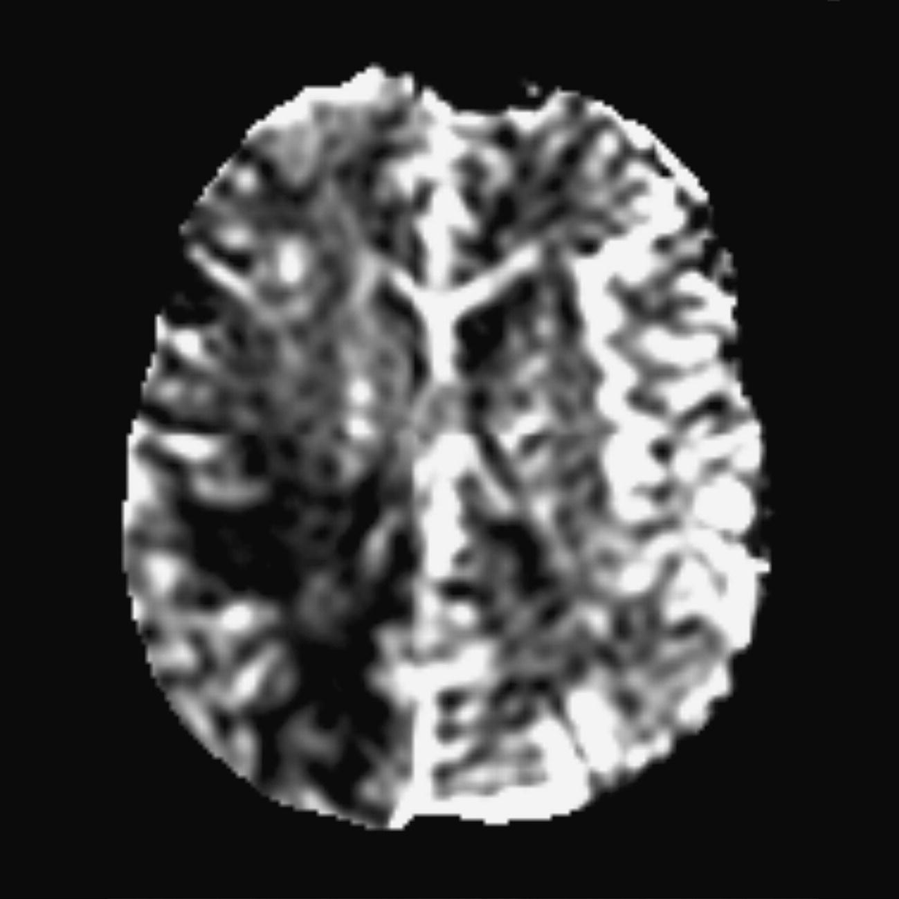
Image optimization
Technical Issues
Artefact problems
Patient considerations
Contrast usage
Temporal lobes
Basic anatomy (Figure 8.21)
Common indications
Equipment
Patient positioning
Suggested protocol
Sagittal SE T1
Axial/oblique SE/FSE T2
Coronal/oblique SE/FSE T1
Coronal 3D incoherent (spoiled) GRE T1 (Figure 8.24)
Axial/oblique/coronal/oblique IR-FSE T2 (Figures 8.25 and 8.26)
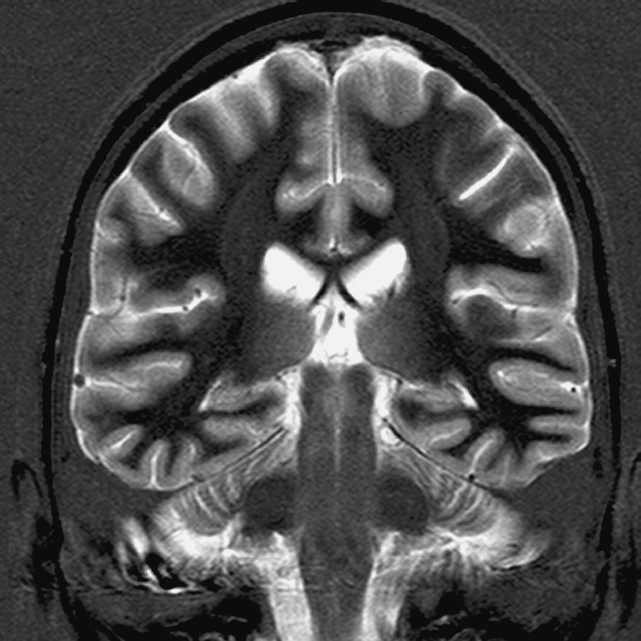
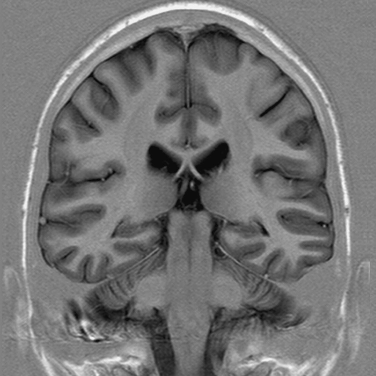
Image optimization
Technical issues
Related posts:


Stay updated, free articles. Join our Telegram channel

Full access? Get Clinical Tree


