The concept of diffusion magnetic resonance imaging (MRI) emerged in the mid-1980s, together with the first images of water molecular diffusion in the human brain, as a way to probe tissue structure. Since then, diffusion MRI has become a pillar of modern clinical imaging. Diffusion MRI is both a method and a powerful concept, because diffusing water molecules provide unique information on the tissue microscopic architecture. Diffusion MRI has initially been used to investigate neurological disorders, aided by amenable conditions of relatively immobile and high T2 signal of the brain. However, further work has shown that diffusion MRI could work in the body as well, and applications are now rapidly expanding in oncology for the detection of malignant lesions and metastases and for monitoring therapy. Water diffusion is significantly decreased in most malignant tissues, and diffusion MRI, which does not require any tracer injection, is rapidly becoming a modality of choice to detect, characterize, or even grade malignant lesions, especially in the prostate and the breast.
Basic Diffusion MRI, Diffusion-Weighted Imaging (DWI), and the Classic Apparent Diffusion Coefficient (ADC)
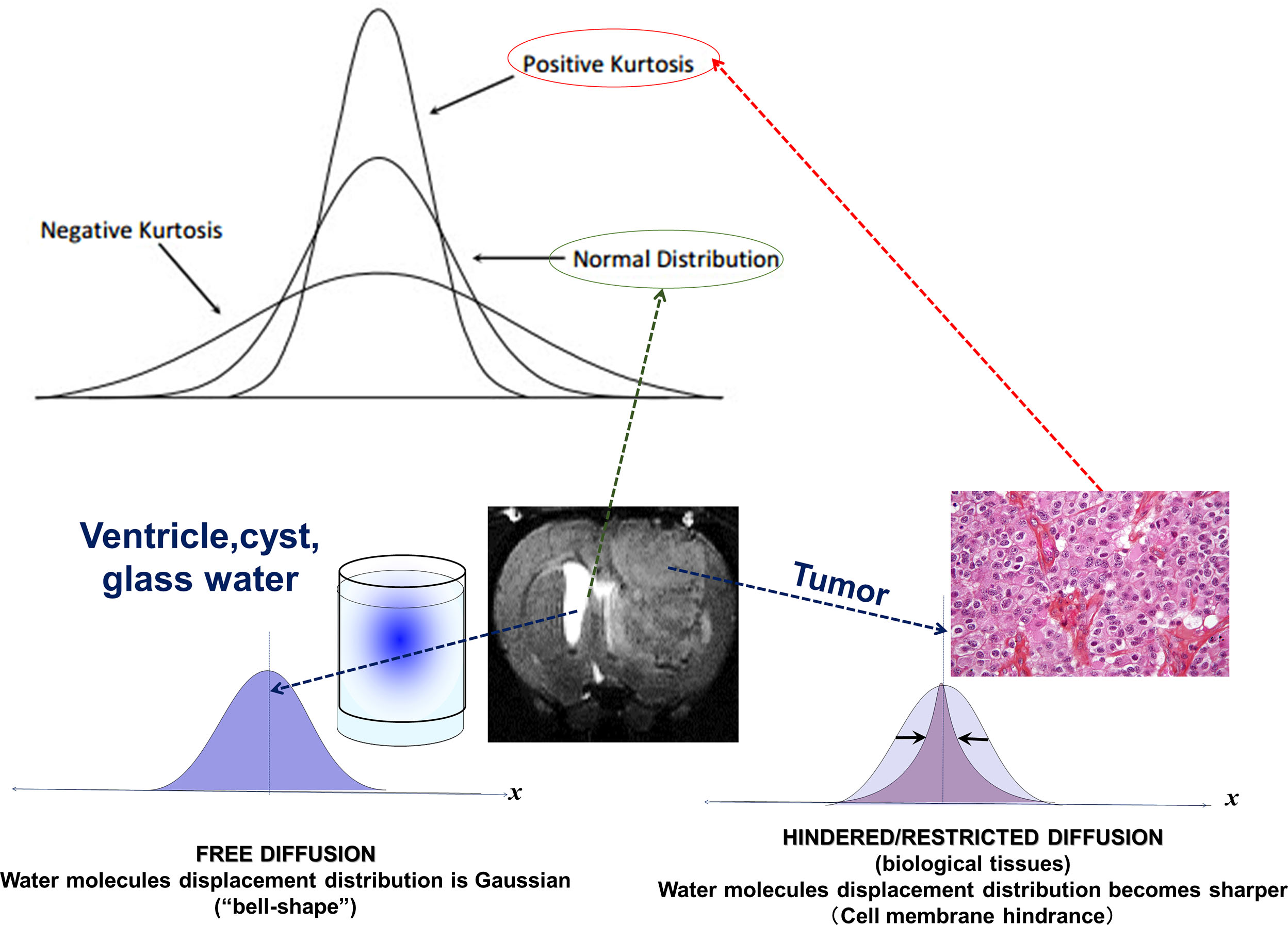
Molecular diffusion refers to the random translational motion of molecules (also called Brownian motion), a physical process that results from the thermal energy carried by these molecules, which was well characterized by Einstein. In a free medium, during a given time interval, molecular displacements obey a 3D Gaussian distribution ( Fig. 1.1 ): molecules travel randomly in space over a distance that is statistically well described by a diffusion coefficient (D). This coefficient depends only on the size (mass) of the molecules, the temperature, and the nature (viscosity) of the medium. For example, in the case of “free” water molecules self-diffusing in water at body temperature (37°C), the diffusion coefficient is 3 × 10 −3 mm 2 /s, which, based on Einstein’s mean displa-cement equation, 6 translates to a mean diffusion distance of 17 μm during 50 ms along one direction ( Fig. 1.1 ). Diffusion MRI is thus deeply rooted in the concept that, during their diffusion-driven displacements, molecules probe tissue structure at a microscopic scale well beyond the usual millimetric image resolution. During typical diffusion imaging times of about 50 to 100 ms, water molecules move in tissues on average over distances around 1 to 15 μm, bouncing, crossing, or interacting with many tissue components, such as cell membranes, fibers, or macromolecules. (The diffusion of other metabolites can also be detected with diffusion MR spectroscopy.) Because of the tortuous movement of water molecules around those obstacles (i.e., “hindered” diffusion; see Fig. 1.1 ), the actual diffusion distance is reduced compared with free water (see Fig. 1.1 ), and the displacement distribution is no longer Gaussian (the shrinkage of the distribution is characterized by a parameter called “kurtosis”). In other words, over very short times, diffusion reflects the local intrinsic viscosity, whereas at longer diffusion times the effects of the obstacles become predominant. Hence, the noninvasive observation of the water diffusion-driven displacement distributions in vivo provides unique clues to the fine structural features and geometrical organization of cells in tissues and to changes in those features with physiological or pathological states.
Imaging Diffusion With MRI
Although early water diffusion measurements were made in biological tissues using nuclear magnetic resonance in the 1960s and 1970 s, it was not until the mid-1980s that the basic principles of diffusion MRI were laid out. By combining MRI principles with those introduced earlier in nuclear magnetic resonance physics and chemistry to encode molecular diffusion effects, it became possible for the first time to obtain local measurements of water diffusion in vivo in the human brain. Contrast underlying standard MRI results from the water hydrogen nuclei (proton) density and the “relaxation times,” called T1 and T2, which characterize how fast water magnetization returns to equilibrium after the perturbation induced by the MRI radiofrequency pulse and which roughly depend on the tissue chemical nature. MRI signals can be sensitized to diffusion through the application of a pair of sharp magnetic field gradient pulses, the duration and the separation of which can be adjusted to achieve a specific level of diffusion sensitization. In an otherwise homogeneous field, the first pulse magnetically labels hydrogen nuclei carried by water molecules according to their spatial location, as for a short time the magnetic field slowly varies along the magnetic field gradient pulse direction ( Fig. 1.2 ). As a result, those nuclei dephase linearly according to their location along this direction. The second pulse is introduced slightly later to exactly rephase nuclei that have not moved. Any nuclei that have changed location due to their diffusion between the two pulses will maintain some degree of phase shift depending on the net nuclei displacement history that occurred during the time interval (or “diffusion time”) between the two pulses. Considering now a population comprising a considerably large number of diffusing water molecules, the overall effect is that the corresponding hydrogen nuclei will experience various phase shifts reflecting the statistical displacement distribution of this population (i.e., the overall diffusion process). This phase distribution contributes to a decrease in the amplitude of the MRI signal compared with that which would be obtained from a population of perfectly stationary nuclei in a perfectly homogeneous field. This signal attenuation is precisely and quantitatively linked to the amplitude of the displacement distribution: fast (slow) diffusion results in a large (small) distribution and a large (small) signal attenuation. Of course, the effect also depends on the intensity of the magnetic field gradient pulses used for this diffusion encoding.
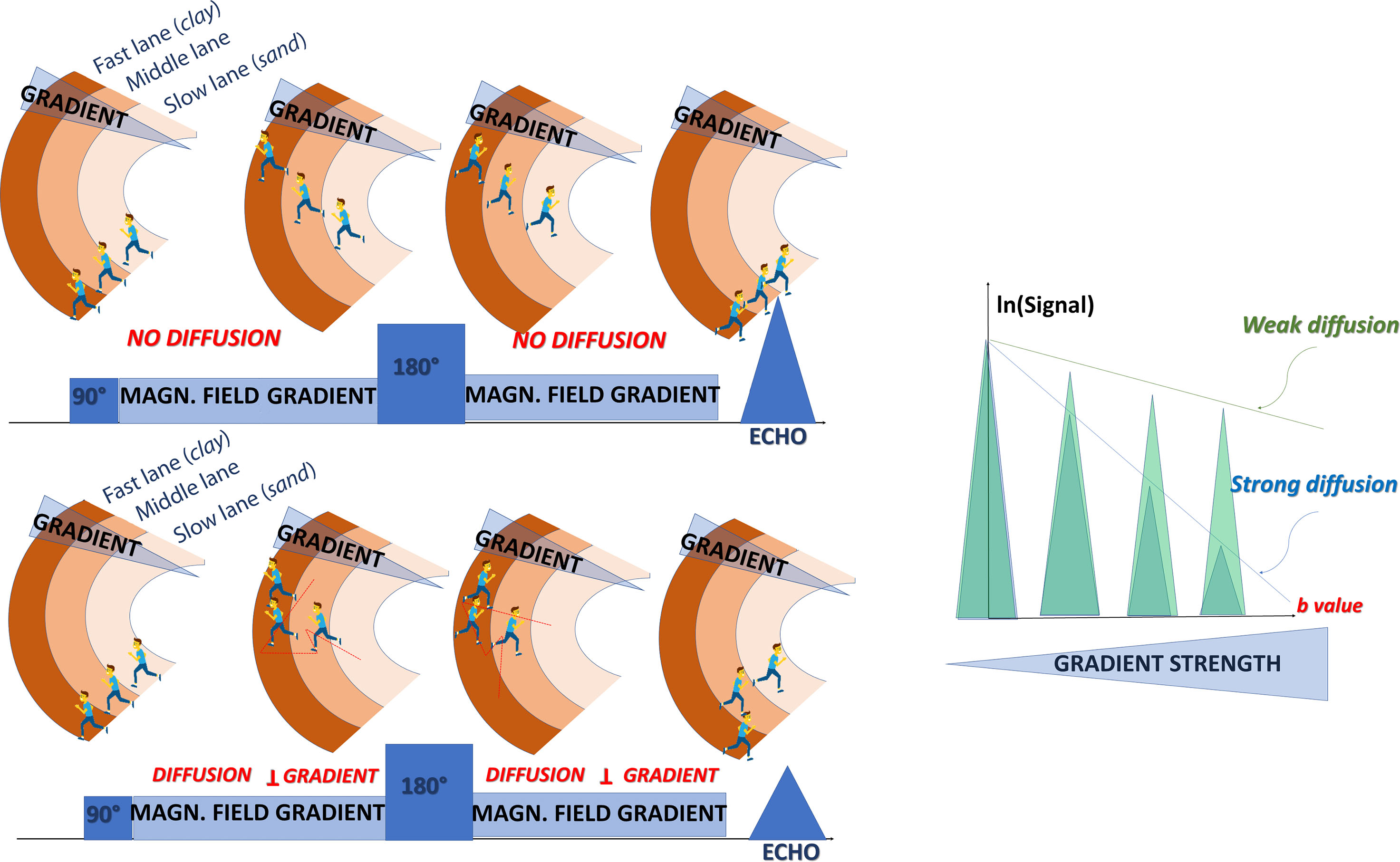
In practice, almost any MRI technique can be sensitized to diffusion by inserting the adequate magnetic field gradient pulses, but the most commonly used in clinical practice is the spin-echo sequence (as illustrated in Fig. 1.2 ). Other sequences, namely, oscillating gradient spin echo (OGSE) and stimulated echo (STEAM) sequences may also be used to access very short or very long diffusion times, respectively. By acquiring data with various gradient pulse amplitudes, one obtains images with different degrees of diffusion sensitivity (see Fig. 1.2 ). The degree of sensitivity to diffusion is described by the so-called b value (usually in s/mm 2 ; typical values are around 1000 s/mm 2 ), which was introduced to take into account the intensity and time profile of the gradient pulses used both for diffusion encoding and MRI spatial encoding. The overall effect of diffusion in the presence of those gradient pulses is a signal attenuation, and the MRI signal becomes diffusion weighted, hence the term “diffusion-weighted imaging” (DWI). The signal attenuation is more pronounced when using large b values and when diffusion is fast. Finally, it is important to notice that only the displacement (diffusion) component along the gradient direction is detectable.
ADC
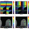
Contrast in these images depends on diffusion, but also on other MRI parameters, such as the water relaxation times T1 and T2, which could lead to well-known artifacts, such as the “T2-shine-through” effect, as lesions with a high T2 signal (e.g., necrosis, cysts) may retain a relatively high signal level at high b values. Hence, these images are often numerically combined to determine, using a global diffusion model, a quantitative estimate of the diffusion coefficient in each image location. The resulting images are maps of the diffusion process and can be visualized using a quantitative scale ( Fig. 1.3 ).
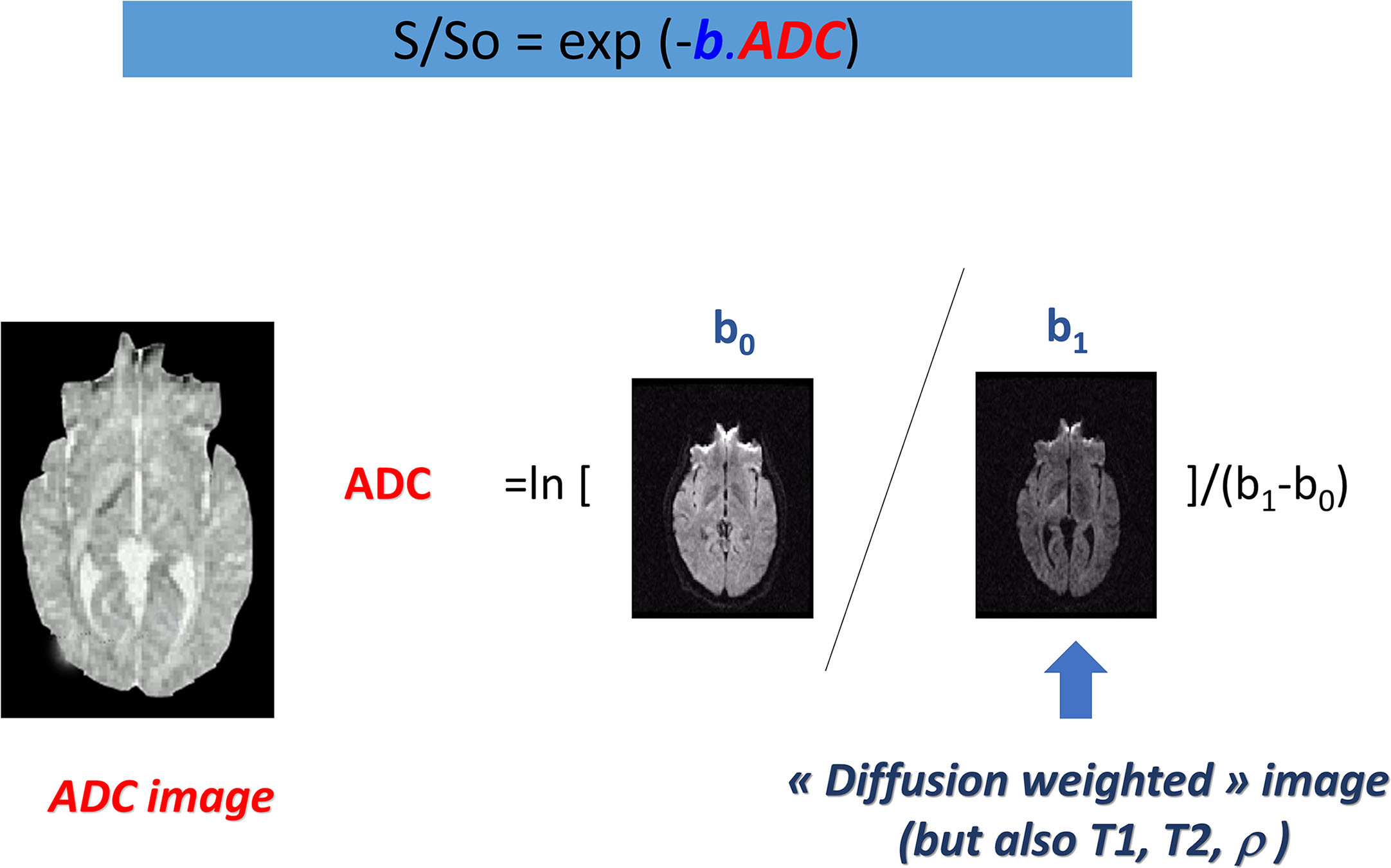
The most basic model is that of the ADC :
ADC=ln[S(b0)−S(b1)]/(b1−b0)
where S(b 0 ) and S(b 1 ) are the signals (in a voxel or a region-of-interest, ROI) acquired at the b values b 0 and b 1 , respectively.
An important point to consider, however, is that Einstein’s equation, which serves as the basis for diffusion MRI, was established for “free” (Gaussian) diffusion, as can be found in a glass of water. In biological tissues, however, diffusion is no longer free, as we have seen (see Fig. 1.1 ). This is indeed what has made diffusion MRI so exquisitely sensitive to tissue structure in various pathological or physiological conditions. As the molecular displacement distribution deviates from a Gaussian law, the diffusion effect on the MRI signal is no longer adequately described by Einstein’s equation. Furthermore, the overall signal observed in a diffusion MRI image volume element (voxel, often larger than 2 mm in size for common breast diffusion MRI) results from the integration, on a statistical basis, of all the microscopic displacement distributions of the water molecules present in this voxel.
For those reasons, as a departure from earlier biological diffusion studies where efforts were made to depict the true diffusion process, the ADC concept was introduced to portray the complex diffusion processes that occur in a biological tissue on a voxel scale using the microscopic , free diffusion physical model. In clinical diffusion MRI, the physical diffusion coefficient (D) is replaced by a global, statistical parameter, the ADC. This parametrization allows us to bridge the gap between the two scales without the need to use sophisticated models. Indeed, this simple ADC has been an incredibly robust and powerful parameter, which has been largely used across all clinical applications of diffusion MRI since its debut.
Beyond the ADC: Advanced Diffusion MRI
Looking at the signal decay with the b value, one immediately sees that the attenuation is not linear but presents a marked curvature, especially at the extremities ( Fig. 1.4 ), at the beginning of the curve (very small b values), and when b values become large (beyond 800 s/mm 2 ). This curvature provides important clues on the underlying tissue properties that can be elucidated by going beyond the classic ADC model. We provide here a short description of the general principles underlying such advanced applications, which will be developed in more detail in the third section of this book.
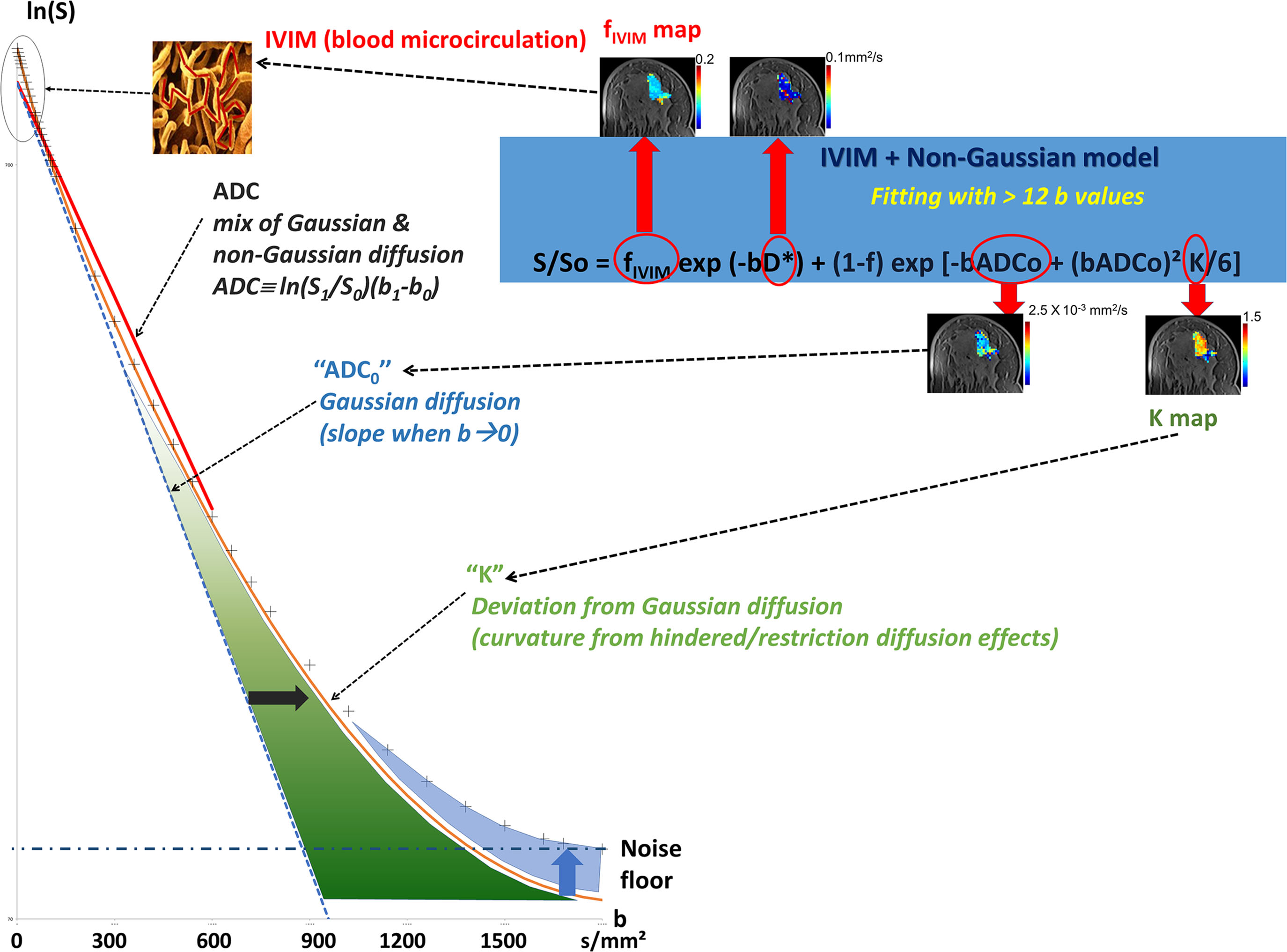
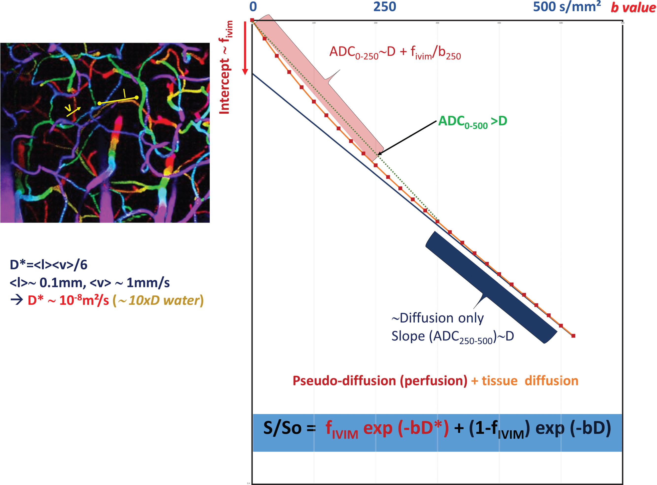
Diffusion MRI at Very Low b Values: IVIM and Perfusion
The ADC concept was introduced to encompass all types of incoherent motions present within each image voxel (hence the abbreviation IVIM for intravoxel incoherent motion), which could contribute to the signal attenuation observed with diffusion MRI. Beyond molecular diffusion, blood microcirculation in the capillary networks (perfusion) also contributes. Indeed, the flow of blood in large vessels passing through voxels can be seen as coherent (hence not affecting diffusion-weighted images), whereas the flow of blood water in randomly oriented capillaries (at voxel level) mimics a random walk (“pseudodiffusion”), which results in a signal attenuation in the presence of the diffusion-encoding gradient pulses. This apparent motion randomness for perfusion results from the geometry of the microvessel network where blood circulates, under the hypothesis that the microvascular network can be modeled by a series of straight segments randomly oriented in space with a uniform angular coverage (4π solid angle) within each voxel. Here, randomness thus results from the collective motion of blood water molecules in the network, flowing from one capillary segment to the next, in addition to the individual diffusion movement of blood water molecules. This collective movement has been described as a pseudodiffusion process where average displacements, l, would now correspond to the mean capillary segment length and the mean velocity, v , would be that of blood in the vessels ( Fig. 1.5 ). In the presence of blood microcirculation the overall MRI signal attenuation, S(b)/S(0), becomes the sum of two exponentials (biexponential decay), one for tissue diffusion and one for the blood compartment (assuming water exchange between blood and tissues is negligible during the encoding time, a hypothesis that has not yet been deeply investigated):
S(b)/S0=fIVIMexp[−b(D*+Dblood)]+(1−fIVIM)exp(−bD)
Related posts:
 Disease and Treatment Monitoring
 Diffusion MRI as a Stand-Alone Unenhanced Approach for Breast Imaging and Screening
 Conventional Breast Imaging
 Diffusion-Weighted Whole Body Imaging With Background Body Signal Suppression (DWIBS)
 Diffusion-Weighted Imaging (DWI) for Breast Lesion Characterization: The Olea Medical Perspective and the Utilization of Olea Sphere Software
 Breast Diffusion MRI Acquisition and Processing Techniques: The GE Healthcare Perspective
Stay updated, free articles. Join our Telegram channel

Full access? Get Clinical Tree


