Hip(I)


10.1055/b-0034-92242

Hip(I)


Radiographic Landmarks of the Hip


The following radiographic landmarks and their interrelationships are helpful in diagnosing congenital and acquired abnormalities of the acetabulum ( Fig. 2.1 ):


  • Iliopectineal line (arcuate line, linea terminalis): The iliopectineal line is the radiographic reference line for the anterior column.


  • Ilioischial line: The upper portion of this line is formed by the posterior part of the quadrilateral plate, its lower portion by the ischium (medial boundary). The ilioischial line is the landmark for the posterior column.


  • Acetabular roof line.


  • Acetabular teardrop: This is a teardrop-shaped figure formed laterally by the medial portion of the acetabulum and medially by the antero-inferior portion of the quadrilateral plate. The quadrilateral plate is the posterior wall of the acetabulum, which faces inward on the pelvic inlet and presents an approximately square, flat surface.


  • Anterior rim of the acetabulum.


  • Posterior rim of the acetabulum.

Armbuster TG, Guerra J Jr, Resnick D, et al. The adult hip: an anatomic study. Part I: the bony landmarks. Radiology 1978;128(1):1–10


Femoral Neck–Shaft Angle and Anteversion Angle


Projected Neck–Shaft Angle

The projected femoral neck–shaft angle (NSA, called also the caput–collum–diaphyseal (CCD) angle; Fig. 2.2 ) is determined on the anteroposterior (AP) pelvic radiograph or the AP radiograph of the hip and femur. It is the angle formed by the longitudinal axes of the neck and shaft of the femur.

Anatomic landmarks for evaluating the hip in the anteroposterior pelvic radiograph. 1 = Iliopectineal line 2 = Ilioischial line 3 = Acetabular roof line 4 = Acetabular teardrop 5 = Posterior rim of acetabulum 6 = Anterior rim of acetabulum a Schematic drawing. b Anteroposterior pelvic radiograph.
Neck–shaft angle. Schematic drawing.

The femoral neck axis can be determined as follows ( Fig. 2.3 ): first the center of the femoral head is located with a circle template or computer-assisted technique at a workstation. Next a line is drawn connecting the points where the circle intersects the medial and lateral borders of the femoral neck. A line drawn perpendicular to that line through the center of the femoral head represents the femoral neck axis.


M.E. Müller uses the following method for an accurate reconstruction of the NSA:


  1. The center of the femoral head is located with a circle template or a computer-assisted technique. Reference points for the circular arc are the lateral portion (outermost point) of the epiphysis and the medial corner of the femoral neck.


  2. The point of deepest concavity on the lateral border of the femoral neck is marked.


  3. Another arc through that point using the center of the femoral head as the center is drawn.


  4. The points where the circle intersects the femoral neck are connected.


  5. A line is drawn perpendicular to that line through the center of the femoral head. That line represents the femoral neck axis.


  6. The femoral shaft axis is drawn midway between the lateral and medial borders of the femoral shaft.


Projected NSA


Normal values in adults:


~ 120–130°


Coxa valga:


> 130°


Coxa vara:


< 120°


The anteversion of the proximal femur causes the NSA to appear larger on radiographs than it really is.

Determining the femoral neck axis on an anteroposterior radiograph of the hip or pelvis. a Approximate determination of the femoral neck axis.

M = Center of the femoral head


A = Point where the circle intersects the lateral cortex of the femoral neck


B = Point where the circle intersects the medial cortex of the femoral neck


1 = Femoral neck axis (line perpendicular to AB through M)


b M. E. Müller method for accurate reconstruction of the femoral neck axis.


M = Center of the femoral head


A = Deepest point in lateral concavity of the femoral neck


B = Point on medial border of the femoral neck defined by the second arc


1 = Femoral neck axis (line perpendicular to AB through M)


2 = Femoral shaft axis

Dunn–Rippstein– Müller method of determining the anteversion angle on conventional radiographs. Schematic illustration. a View from the foot of the table. b Side view.
Dunn-Rippstein-Müller method of reconstructing the anteversion angle. M = Center of the femoral head A = Deepest point in lateral concavity of the femoral neck B = Point where the second arc intersects the medial femoral neck

1 = Femoral neck axis (line perpendicular to AB through M)


2 = Horizontal plane (defined by the positioning frame)


3 = Projected anteversion angle

Müller ME. Die hüftnahen Femurosteotomien. 1st ed. Stuttgart: Thieme; 1957


Projected Anteversion Angle (Dunn–Rippstein–Müller Method)

Today the Dunn–Rippstein–Müller method is widely used to assess rotational deformity by calculating the true NSA and femoral anteversion (AV) angle. The projected AV angle is measured on a radiograph in the Rippstein projection (called also the Rippstein II view). This projection is standardized by using a positioning frame that holds the hip in 90° of flexion and 20° of abduction ( Fig. 2.4 ).


The AV angle is measured between the horizontal plane (defined by the positioning frame) and the femoral neck axis ( Fig. 2.5 ). The Müller method (see p. 11) is best for determining the femoral neck axis. When calculated in this way, the AV angle is determined relative to the transverse axis of the femoral condyles.


True Neck–Shaft Angle and Anteversion Angle

Geometric formulae are available for converting the projected NSA and AV angle to the true angles.


Calculation of the true AV angle:


Calculation of the true NSA:


cot β = cot β2 • cot α


where:


α = true AV angle


α2 = projected AV angle


β2 = projected NSA


γ = abduction angle of the femur = 20°


The use of conversion charts will facilitate the rapid calculation of values in everyday practice. The chart published by Müller in 1957 is a well-established clinical tool ( Table 2.1 ). Another current option is the use of computer software.


Both the NSA and AV angle change with aging and show a large range of variation. Tables 2.2 and 2.3 list age-adjusted normal values and analytic criteria proposed by the Commission for the Study of Developmental Dysplasia of the Hip of the German Society for Orthopedics and Traumatology. These tables can be helpful in routine clinical decision-making. Prognostic assessments are difficult, however, because spontaneous normalization often occurs during growth and cannot be predicted with certainty.


Chart for finding the true values of the anteversion (AV) angle (horizontal numbers) and neck–shaft angle (NSA) (vertical numbers) based on the projected angles (source: Müller 1957)

Projected AV angle (°)


5


10


15


20


25


30


35


40


45


50


55


60


65


70


75


80


Projected NSA (°)


100


4


9


15


20


25


30


35


40


45


50


55


60


65


70


75


80


101


100


100


100


100


99


99


98


97


96


95


94


94


93


92


91


105


5


9


15


20


25


31


35


41


46


51


56


60


65


70


75


80


105


105


104


104


103


103


102


100


100


99


98


97


96


95


94


92


110


5


10


16


21


27


32


36


42


47


52


56


61


66


71


76


80


110


110


109


108


108


106


106


105


104


103


101


99


98


97


95


93


115


5


10


16


21


27


32


37


43


48


52


57


62


67


71


76


81


115


115


114


112


112


111


110


109


107


105


104


102


101


99


96


94


120


6


11


16


22


28


33


38


44


49


53


58


63


68


72


77


81


120


119


118


117


116


115


114


112


110


108


106


104


103


101


98


95


125


6


11


17


23


28


34


39


44


50


54


58


63


68


72


77


81


125


124


123


121


120


119


118


116


114


112


109


107


105


103


100


95


130


6


12


18


24


29


35


40


46


51


55


60


64


69


73


78


82


130


129


127


126


125


124


122


120


117


116


112


109


107


104


101


96


135


7


13


19


25


31


36


42


47


52


56


61


65


70


74


78


82


135


133


132


131


130


129


126


124


120


118


114


112


109


105


102


96


140


7


13


20


27


32


38


44


49


53


58


63


67


71


75


79


83


139


138


137


135


134


132


130


127


124


120


117


114


111


107


103


97


145


8


14


21


28


34


40


45


50


55


59


64


68


72


75


79


83


144


142


141


139


138


136


134


131


128


124


120


117


114


110


104


98


150


8


15


22


29


35


42


47


52


56


61


65


69


73


76


80


84


149


147


146


144


143


141


138


136


134


129


124


120


116


112


105


100


155


9


17


24


32


38


44


50


54


58


63


67


71


74


77


81


84


154


152


151


149


148


145


142


139


137


132


128


124


119


115


108


103


160


10


18


27


34


44


46


52


57


61


65


69


73


76


79


82


82


159


158


157


155


153


151


147


144


141


134


132


128


122


116


111


105


165


13


23


33


40


47


53


57


62


67


69


73


76


78


81


83


86


164


162


160


159


158


156


153


148


144


140


135


130


122


119


113


106


170


15


27


37


46


53


58


63


67


70


73


76


78


80


83


84


87


169


167


166


164


163


159


157


154


150


145


142


134


130


122


118


113

Dunn DM. Anteversion of the neck of the femur; a method of measurement. J Bone Joint Surg Br 1952;34-B (2):181–186 Müller ME. Die hüftnahen Femurosteotomien. 1st ed. Stuttgart: Thieme; 1957 Rippstein J. Determination of the antetorsion of the femur neck by means of two x-ray pictures. [Article in German] Z Orthop Ihre Grenzgeb 1955;86(3):345–360 Tönnis D. Die angeborene Hüftdysplasie und Hüftluxation im Kindes- und Erwachsenenalter. Chapter 9: Allgemeine Röntgendiagnostik des Hüftgelenks. Berlin: Springer; 1984; 129–134


Classification of true neck–shaft angles (NSAs) (Commission for the Study of DDH, German Society for Orthopedics and Traumatology; MV = mean value; source: Tönnis 1984)

Age (years)


Grade –4 (extremely abnormal)


Grade –3 (severely abnormal)


Grade –2 (slightly abnormal)


Grade 1 (normal to borderline)


Grade +2 (slightly abnormal)


Grade +3 (severely abnormal)


Grade +4 (extremely abnormal)


> 1 to < 3


< 105


≥ 105 to < 115


≥ 115 to < 125


≥ 125 to < 150 (MV 140)


≥ 150 to < 155


≥ 155 to < 160


≥ 160


> 3 to < 5


< 105


≥ 105 to < 115


≥ 115 to < 125


≥ 125 to < 145 (MV 135)


≥ 145 to < 150


≥ 150 to < 155


≥ 155


> 5 to < 10


< 100


≥ 100 to < 110


≥ 110 to < 120


≥ 120 to < 145 (MV 132)


≥ 145 to < 150


≥ 150 to < 155


≥ 155


> 10 to < 14


< 100


≥ 100 to < 110


≥ 110 to < 120


≥ 120 to < 140 (MV 130)


≥ 140 to < 145


≥ 145 to < 155


≥ 155


14 or more


< 100


≥ 100 to < 110


≥ 110 to < 120


≥ 120 to < 135 (MV 128)


≥ 135 to < 140


≥ 140 to < 150


≥ 150


Classification of true anteversion (AV) angles (Commission for the Study of DDH, German Society for Orthopedics and Traumatology; MV = mean value; source: Tönnis 1984)

Age (years)


Grade –4 (extremely abnormal)


Grade –3 (severely abnormal)


Grade –2 (slightly abnormal, borderline)


Grade 1 (normal)


Grade +2 (slightly abnormal, borderline)


Grade +3 (severely abnormal)


Grade +4 (extremely abnormal)


> 1 to < 3


< 20


≥ 20 to < 25


≥ 25 to < 35


≥ 35 to < 55 (MV 45)


≥ 55 to < 60


≥ 60 to < 75


≥ 75


≥ 3 to < 7


< 15


≥ 15 to < 20


≥ 20 to < 30


≥ 30 to < 50 (MV 40)


≥ 50 to < 55


≥ 55 to < 70


≥ 70


≥ 7 to < 9


< 10


≥ 10 to < 15


≥ 15 to < 25


≥ 25 to < 45 (MV 35)


≥ 45 to < 50


≥ 50 to < 65


≥ 65


≥ 9 to < 11


< 5


≥ 5 to < 10


≥ 10 to < 20


≥ 20 to < 40 (MV 30)


≥ 40 to < 45


≥ 45 to < 60


≥ 60


≥ 11 to < 13


< 5


≥ 5 to < 10


≥ 10 to < 15


≥ 15 to < 35 (MV 25)


≥ 35 to < 40


≥ 40 to < 55


≥ 55


≥ 13 to <15


< 0


≥ 0 to < 5


≥ 5 to < 10


≥ 10 to < 30 (MV 20)


≥ 30 to < 35


≥ 35 to < 50


≥ 50


≥ 15


< 0


≥ 0 to < 5


≥ 5 to < 10


≥ 10 to < 25 (MV 15)


≥ 25 to < 30


≥ 30 to < 45


≥ 45

Only gold members can continue reading. Log In or Register to continue

Stay updated, free articles. Join our Telegram channel

Jun 21, 2020 | Posted by in MUSCULOSKELETAL IMAGING | Comments Off on Hip(I)

Full access? Get Clinical Tree

Get Clinical Tree app for offline access