Hip(II)

10.1055/b-0034-92243

Hip(II)

Radiographic Evaluation after 4 Years of Age

Center-edge (CE) Angle of Wiberg (Lateral Coverage)

The CE angle is calculated on the AP pelvic radiograph ( Fig. 2.27 ). It is measured between a line parallel to the longitudinal body-axis and a line connecting the center (C) of the femoral head to the outer edge (E) of the superior acetabular rim.

CE angle of Wiberg

Mean values:
- Age 5–8 years: ~ 25°
- Age 9–12 years: ~ 30°
- Age > 12 years: ~ 35°
Normal values:
- Age 5–8 years: > 20°
- Age ≥ 9 years: > 25°

Normal value studies have been performed in various populations. The Commission for the Study of DDH of the German Society for Orthopedics and Traumatology compiled the normal values and grades of deviation shown in Table 2.9 . The CE angle describes the position of the femoral head in relation to the acetabulum. The deeper the acetabulum, the greater the CE angle. As the acetabulum becomes flatter and steeper (dysplastic), the CE angle decreases.

The CE angle is of key importance in evaluating hip dysplasia and is considered the principal angle for evaluating residual hip dysplasia in children and adults.

C = Center of the femoral head

E = Edge of the superior acetabular rim

Tönnis D. Die angeborene Hüftdysplasie und Hüftluxation im Kindes- und Erwachsenenalter. Chapter 9: Allgemeine Röntgendiagnostik des Hüftgelenks. Berlin: Springer; 1984; 129–134 Wiberg G. Studies on dysplastic acetabula and congenital subluxation of the hip joint: with special reference to the complication of osteoarthritis. Acta Chir Scand 1939;58(Suppl.):7–38

VCA Angle of Lequesne and De Sèze

The VCA angle, which reflects the anterior coverage of the femoral head, is measured in the false profile view ( Fig. 2.28 ). This radiograph is taken in the standing position with the pelvis rotated 65° relative to the cassette. The foot is parallel to the film cassette, and weight is borne on the affected leg. The central beam is directed to the femoral head ( Fig. 2.29 ). The VCA angle is formed by a vertical line (V, parallel to the longitudinal body-axis) drawn through the center of the femoral head and an oblique line drawn from the femoral head center to the anterior rim of the acetabulum (A; see Fig. 2.28 ).

V = Vertical line through femoral head center (parallel to longitudinal body axis)

C = Center of the femoral head

A = Anterior border of the acetabulum

VCA angle in adults


• Normal values:	> 25°
• Slightly abnormal:	20° ≤ VCA angle ≤ 25°
• Severely abnormal:	< 20°

The VCA angle is used to evaluate the anterior coverage of the femoral head by the acetabulum. It can detect deficient anterior coverage, which is usually less pronounced than the lateral component of hip dysplasia, as well as very rare instances of isolated anterior dysplasia. In measuring the angle, it may be difficult to identify point A owing to the difficulty of locating the most anterior point of the acetabular roof.

Lequesne M; de Sèze S. False profile of the pelvis. A new radiographic incidence for the study of the hip. Its use in dysplasias and different coxopathies. [Article in French] Rev Rhum Mal Osteoartic 1961;28:643–652

ACM Angle of Idelberger and Frank

The ACM angle is calculated on the AP pelvic radiograph. Several points are identified in constructing this angle ( Fig. 2.30 ).

Positioning technique for the false profile view.

ACM angle

Mean value in adults (according to Busse): 45° ± 3°
Abnormal by approximately age 4: > 50°

The Commission for the Study of DDH of the German Society for Orthopedics and Traumatology published the normal values and grades of deviation for the ACM angle shown in Table 2.10 .

The ACM angle reflects the depth of the acetabulum. Large angles denote a very shallow acetabulum (dysplasia), while small angles mean that the acetabulum has a spherical or hemispherical shape. One advantage of the ACM angle is that it is relatively independent of pelvic tilt and rotation. One disadvantage is that it gives no information on the inclination of the acetabulum relative to the horizontal plane.

Idelberger K, Frank A. A new method for determination of the angle of the pelvic acetabulum in child and in adult. [Article in German] Z Orthop Ihre Grenzgeb 1952;82(4):571–577 Tönnis D. Die angeborene Hüftdysplasie und Hüftluxation im Kindes- und Erwachsenenalter. Chapter 9: Allgemeine Röntgendiagnostik des Hüftgelenks. Berlin: Springer; 1984; 129–134

ACM Angle of Idelberger and Frank. A = Superior rim of the acetabulum B = Inferior rim of the acetabulum M = Midpoint of connecting line AB C = Point on the acetabulum intersected by a line perpendicular to AB and through M α = ACM angle (formed by AC and CM)

Classification of ACM angles (Commission for the Study of DDH, German Society for Orthopedics and Traumatology; source: Tönnis 1984)
Age (years)	Normal mean value	Grade 1 (normal)	Grade 2 (slightly abnormal)	Grade 3 (severely abnormal)	Grade 4 (extremely abnormal)
> 2	45	< 50	≥ 50 to < 55	≥ 55 to < 60	≥ 60

Summarized Hip Factor

The summarized hip factor (SHF, Fig. 2.31 ) is a combination of several values used to make a more accurate prognosis of hip dysplasia. The SHF is calculated on the AP pelvic radiograph. Points A, B, C, M and Z are defined as in the measurement of the ACM angle (see Fig. 2.30 ).

The following formula is used to calculate the SHF:

SHF = A + B + C + 10

where

and ACM = ACM angle, CE = CE angle, MZ = off-center distance (mm).

The mean values and standard deviations in Table 2.11 can be used to calculate the SHF from the above formula (using computer software or a pocket calculator).

For routine clinical work, the SHF can be quickly determined from age-adjusted nomograms (see Appendix to this Chapter, pp. 48 and 49). First calculate the ACM and CE angles and mark them on the two scales on the left side of the nomogram. Draw a connecting line between those points and extend it across the center scale. Next draw a second line connecting that point on the center scale to the off-center distance MZ marked on the fourth scale. The point where that line crosses the right-hand scale will indicate the summarized hip factor.

Mean values and standard deviations for calculating the summarized hip factor (source: Tönnis 1984)
Age (years)	Measurements	Number	Mean value ± standard deviation	Normal range
5 through 8	ACM angle	326	45.9° ± 2.7°	<49°
	CE angle	326	24.7° ± 6.3°	>20°
	MZ distance	326	3.2 mm ± 1.7 mm	<5 mm
9 through 12	ACM angle	326	45.0° ± 2.4°	<46°
	CE angle	326	31.3° ± 5.0°	>26°
	MZ distance	326	2.9 mm ± 1.5 mm	<4 mm
13 through 16	ACM angle	254	45.6° ± 2.8°	<47°
	CE angle	254	34.3° ± 5.7°	>30°
	MZ distance	254	3.1 mm ± 1.5 mm	<5 mm
17 through 20	ACM angle	204	44.6° ± 3.0°	<47°
	CE angle	204	35,1° ± 5.4°	>30°
	MZ distance	204	3.6 mm ± 1.5 mm	<6 mm
21 through 50	ACM angle	358	45.0° ± 3.2°	<49°
	CE angle	358	35.7° ± 6.5°	>30°
	MZ distance	358	3.9 mm ± 1.7 mm	<6 mm
ACM = Angle of Idelberger and Frank CE = Center-edge MZ = Off-center distance

Classification of the summarized hip factor (Commission for the Study of DDH, German Society for Orthopedics and Traumatology; source: Tönnis 1984)
Age (years)	Normal mean value	Grade 1 (normal)	Grade 2 (slightly abnormal)	Grade 3 (severely abnormal)	Grade 4 (extremely abnormal)
≥ 5 to ≤ 18	10	≥ 6 to < 15	≥ 15 to < 20	≥ 20 to < 30	≥ 30
Adults	10	≥ 6 to < 16	≥ 16 to < 21	≥ 21 to < 31	≥ 31

Summarized hip factor

Mean values:
- Children ≥ 5 to ≤ 18 years: 10
- Adults: 10
Normal values:
- Children ≥ 5 to ≤ 18 years: 6 ≤ SHF < 15
- Adults: 6 ≤ SHF < 16

Table 2.12 lists the ranges of values for grading the SHF based on data from the Commission for the Study of DDH.

The SHF takes into account several aspects that are important for age-appropriate development of the joint. The ACM angle reflects the depth of the acetabulum, while the CE angle indicates coverage. The off-center distance MZ measures how far the center point of the femoral head has decentered from the acetabulum.

Calculation of the SHF is relatively complex, so it is not routinely included in the follow-up of known DDH. The advantage of the SHF is that “false-positives” for preosteoarthritic deformity are much less common than when the CE angle, for example, is calculated alone.

Tönnis D. Die angeborene Hüftdysplasie und Hüftluxation im Kindes- und Erwachsenenalter. Chapter 9: Allgemeine Röntgendiagnostik des Hüftgelenks. Berlin: Springer; 1984; 129–134 Tönnis D. Normal values of the hip joint for the evaluation of X-rays in children and adults. Clin Orthop Relat Res 1976;119(119):39–47

Radiographic Measurements after Skeletal Maturity (Residual Hip Dysplasia)

The CE angle of Wiberg (lateral coverage; see Fig. 2.27 ) and the VCA angle of Lequesne and De Sèze (see Fig. 2.28 ) are useful parameters in patients who have reached skeletal maturity. The acetabular angle of Sharp ( Fig. 2.26 ) also plays a key role. Other important values are described below.

Horizontal Toit Externe (HTE) Angle (Acetabular Index of the Weight-Bearing Zone)

The HTE angle ( Fig. 2.32 ) is measured on the AP pelvic radiograph. It reflects the slope of the sclerotic zone of the acetabular roof (weight-bearing surface) relative to the horizontal plane. A line is drawn tangent to the acetabular roof, passing through the most lateral and inferior points of the sclerotic zone. Then a horizontal line is drawn through the lowest point of both sclerotic zones. The angle formed by the two lines is the HTE angle.

HTE angle

Normal value in adolescents and adults: – 10° to + 10°
Tschauner classification of the HTE angle:
- Grade 1 (normal): < 9°
- Grade 2 (slightly abnormal): 10–15°
- Grade 3 (severely abnormal): 16–25°
- Grade 4 (extremely abnormal): > 25°

Horizontal toit externe angle of the acetabular weight-bearing zone.

The acetabular index can no longer be determined after the triradiate cartilage has closed, but the sclerotic weight-bearing zone of the acetabular roof can still be seen on conventional radiographs. Its slope is of great functional importance because only a near-horizontal orientation of the weight-bearing surface will allow uniform pressure transfer across the joint.

CT Measurement of Acetabular Coverage

The degree of femoral head coverage by the acetabulum can be evaluated on transverse CT images using a technique established by Anda et al ( Fig. 2.33 ). The measurement is performed on a transverse CT section acquired through the centers of both femoral heads. The center points (Z) are located with a circle template or a computer-assisted technique and interconnected by a straight line (g).

From the center of each femoral head, a line is drawn tangent to the anterior and posterior rims of the acetabulum. The angle formed by the tangent to the anterior acetabular rim and the line connecting the femoral head centers (g) is called the anterior acetabular sector angle (AASA). Similarly, the tangent to the posterior acetabular rim forms the posterior acetabular sector angle (PASA). The AASA quantifies the anterior coverage of the femoral head, while the PASA quantifies its posterior coverage. The sum of both angles, called the horizontal acetabular sector angle (HASA), provides a parameter for assessing global acetabular coverage. Normal values for the AASA, PASA and HASA are shown in Table 2.13 .

Quantification of femoral head coverage on transverse computed tomography sections.

Z = Center of the femoral head

A = Anterior rim of the acetabulum

P = Posterior rim of the acetabulum

g = Straight line through the femoral head centers

AASA = Anterior acetabular sector angle

PASA = Posterior acetabular sector angle

HASA = Horizontal acetabular sector angle

Normal values for the anterior, posterior and horizontal acetabular sector angles
	Men	Women
AASA	64° ± 6°	63° ± 6°
PASA	102° ± 8°	105° ± 8°
HASA	167° ± 11°	169° ± 10°
AASA = Anterior acetabular sector angle PASA = Posterior acetabular sector angle HASA = Horizontal acetabular sector angle

Anda S, Svenningsen S, Dale LG, Benum P. The acetabular sector angle of the adult hip determined by computed tomography. Acta Radiol Diagn (Stockh) 1986;27(4):443–447 Anda S, Terjesen T, Kvistad KA. Computed tomography measurements of the acetabulum in adult dysplastic hips: which level is appropriate? Skeletal Radiol 1991;20(4):267–271 Anda S, Terjesen T, Kvistad KA, Svenningsen S. Acetabular angles and femoral anteversion in dysplastic hips in adults: CT investigation. J Comput Assist Tomogr 1991;15(1):115–120

Perthes Disease

Perthes disease refers to aseptic (idiopathic) osteonecrosis of the femoral head in children. Its course differs markedly from osteonecrosis of the femoral head in adults owing to the high healing potential in the pediatric age group.

Stages of the Disease (Waldenström Stages)

Perthes disease passes through five consecutive stages, first described by H. Waldenström:

Initial stage: cessation of growth of the capital femoral epiphysis
Condensation: sclerosis of the epiphysis with initial subchondral fracture
Fragmentation (resorption)
Reossification (repair)
Healing

Catterall Classification

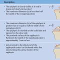
The extent of epiphyseal necrosis and metaphyseal involvement significantly affect the prognosis of Perthes disease. In 1971 Catterall introduced a radiographic classification that quantifies the extent of epiphyseal necrosis and assigns patients to prognostic groups ( Fig. 2.34 ). The Catterall classification is based on conventional radiographs: the AP view and the frog lateral view (Lauenstein view). Patients in groups 1 and 2 have a good prognosis without treatment (> 90% of cases), but the prognosis for untreated patients in groups 3 and 4 is poor (> 90% of cases).

Besides the Catterall classification, the Herring and Salter–Thompson classification systems also quantify the extent of epiphyseal involvement and supply a corresponding prognosis. The Catterall classification is the most widely used, however. It is generally agreed that hips in Catterall groups 3 and 4, Salter–Thompson group B, or Herring group C have an unfavorable prognosis and therefore require treatment.

Only gold members can continue reading. Log In or Register to continue