Image Construction: Part II (Spatial Encoding)
Introduction
In the last chapter, we learned how to select a slice and how to adjust its thickness. However, we did not address the question of from where within a particular slice each component of the signal comes. In other words, we still don’t have spatial information regarding each slice. To create an image of a slice, we need to know how much signal comes from each pixel (picture element) or, more accurately, each voxel (volume element). This is the topic of spatial encoding, of which there are two parts: (i) frequency encoding and (ii) phase encoding.
Frequency Encoding
After selecting a slice, how can we get information about individual pixels within that slice? As an example, consider a slice with three columns and three rows, for a total of 9 pixels. This slice is selected using a selective 90° pulse (Fig. 11-1). We turn the Gz (slice-select gradient) on during the 90° pulse and turn it off after the 90° pulse.
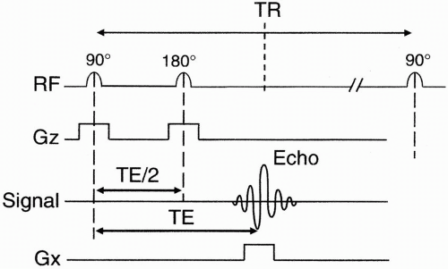 Figure 11-1. Spin-echo pulse sequence diagram. |
We also send a selective 180° RF refocusing pulse, and we again turn the Gz gradient on during the 180° pulse. The echo is received after a time TE. The echo is a signal from the entire slice. To get spatial information in the x direction of the slice, we apply another gradient Gx called the frequency-encoding gradient (also called the readout gradient) in the x direction (Fig. 11-2). With this gradient in the x direction, the center of this 3 × 3 matrix (the center volume) is not going to experience the gradient, that is, it’s not going to experience any change in magnetic field from that prior to turning on the Gx gradient. The column of pixels to the right of midline will experience a higher net magnetic field. The column of pixels on the left will have a lower net magnetic field.
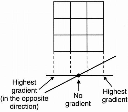 Figure 11-2. Frequency-encoding gradient along the x-axis. |
The Gx gradient is applied during the time the echo is received, that is, during readout.
Let’s now assign some magnitude numbers to the pixels in the matrix (Fig. 11-3).
The numbers in each pixel and their specific location is what we ultimately want to discover because this corresponds to an image. We want to recreate this image using MRI.
Initially, all the protons in this section experience the same frequency of precession. Let’s call that frequency ω0. Now let’s assign each pixel its frequency at a specific point in time before turning on the Gx gradient, while they all still have the same frequency, and combine it with the magnitude we’ve assigned to each pixel (Fig. 11-4). For simplicity, we’ll use a cosine wave as the received signal. In reality, the received signal is a more complicated one, such as a sinc wave.
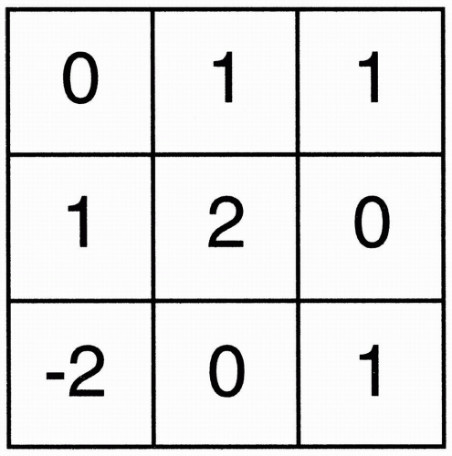 Figure 11-4. Each pixel is also assigned a frequency ω0 and is represented as A cos ω0t, where A is the magnitude. |
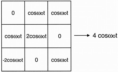 Figure 11-3. In the previous example of a 3 × 3 matrix, each pixel is assigned a value (magnitude). |
Each pixel has a designated magnitude (amplitude), and they all have the same precessional frequency ω0 (except those pixels that have zero signal amplitude). Without any gradient in the x direction, this is the signal we’re going to get. The signal will be the sum of all the signals from each pixel.
The sum of the amplitudes = (0) + (1) + (-2) + (1) + (2) + (0) + (1) + (0) + (1) = 4 The frequency is the same for each pixel (i.e., ω0), as is the shape of the signal (i.e., cos ω0t). So the sum of the pixels = signal from whole slice = 4 cos ω0t We know that, in reality, the signal is more complex. For example, the signal is a decaying signal with time such as a sinc wave, but, for simplicity, let’s accept that we are dealing with
a simple cosine wave as our signal with an amplitude of 4.
a simple cosine wave as our signal with an amplitude of 4.
In summary, when we transmit an RF pulse with frequencies appropriate for a particular slice, all the protons in that slice will start to precess in phase at the Larmor frequency (ω0). Each pixel contains a different number of protons designated by a number. For purposes of illustration, the number we have assigned to each pixel is proportional to the number of protons in each pixel. This number corresponds to the amplitude of the signal. The signal is designated as a cosine wave because it oscillates as a result of the precessing protons. However, we still do not have any spatial information; all we have at this point is a signal coming from the entire slice without spatial discrimination. What we want to be able to do is to separate the summed signal into its components and to tell, pixel by pixel, where each component of the received signal originated.
Let’s now apply the frequency-encoding gradient in the x direction and see what happens to the pixels (Fig. 11-5). Let’s look at the three columns in the matrix:
The pixels in the center column will not feel the gradient. Thus, they will remain with the same frequency (ω0). (And, of course, the amplitude of each pixel is constant because the number of protons doesn’t change.)
The column of pixels to the right of midline is going to have slightly higher frequency. We’ll call this (ω0+). This is because at a higher magnetic field strength, the protons in this column will oscillate at a higher frequency.
The column of pixels to the left of midline will experience a slightly lower field strength and thus have a precessional frequency a little lower than the other columns. We’ll call this (ω0–).
The signal that we get now is still the sum of all the individual signals; however, now each column of pixels has a different frequency, so we can algebraically only add up the ones that have the same frequency, as follows: Column #1: 0 + (cos ω0−t) + (−2 cos ω0−t) = −cos ω0−t Column #2: (cos ω0t) + (2 cos ω0t) + 0 = 3 cos ω0t Column #3: (cos ω0+t) + 0 + (cos ω0+t) = 2 cos ω0+t
Sum of signals = (−cos ω0–t) + (3 cos ω0t) + (2 cos ω0+t)
Let’s look at the Fourier transform of the signal before the Gx gradient is applied (Fig. 11-6A) and look at it again after the Gx gradient is applied (Fig. 11-6B). For a cosine wave, the Fourier transform is a symmetric pair of spikes at the cosine frequency, with an amplitude equal to the magnitude of the signal. (Remember that this is simplified. Usually, we deal with a band of frequencies, i.e., the bandwidth, as opposed to a single frequency. However, right now, for simplicity, we leave it as a single frequency, with its Fourier transform as a single spike.)
Now the computer can look at the Fourier transform and see that we are now dealing with three different frequencies:
The center frequency comes from the central column, and the amplitude of the frequency spike represents the sum of the amplitudes of the pixels in that column, that is, (3 cos ω0t).
The higher frequency comes from the column to the right, and the amplitude of that frequency spike represents the sum of the amplitude of the pixels in that column, that is, (2 cos ω0+t).
The lower frequency comes from the column to the left, and the amplitude of that frequency spike represents the sum of the amplitude of the pixels in that column, that is, (−cos ω0−t).
The way frequency encoding works is that frequency and position have a one-to-one relationship:
frequency ↔ position
So far we have done some spatial encoding and have extracted some information from the slice.
We are now able to decompose the slice matrix into three different columns (Fig. 11-7). That is, we have three different shades of gray corresponding to the three columns.
We are now able to decompose the slice matrix into three different columns (Fig. 11-7). That is, we have three different shades of gray corresponding to the three columns.
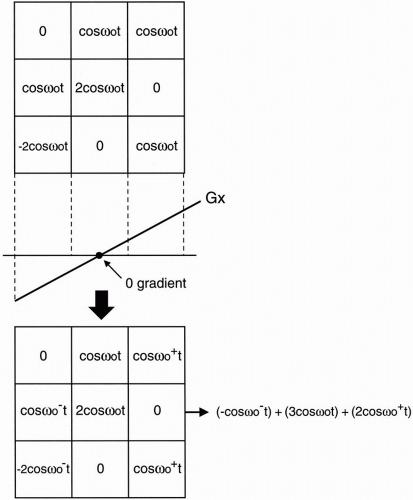 Figure 11-5. When the matrix is exposed to the frequency gradient, different frequencies result in each column: ω0, ω0+, and ω0−. |
So, now we’ve done our job in the x direction. The next thing we want to do is to decompose the individual columns into their three individual pixels (i.e., work in the y direction). The two ways of doing this are as follows:
Back projection
Two-dimensional Fourier transform (2DFT)
Back Projection. If we think in terms of CT imaging and apply gradients, we start out with an area we want to image and apply a gradient (Fig. 11-8A). Then we can rotate the gradient by an angle θ and reapply the gradient (Fig. 11-8B). We can continue this to complete 360°, and
each time we do this we get different numbers. At the end, we end up with a set of equations, which can be solved for values of the pixels in the matrix. This is the back projection approach performed by rotating the frequency gradient.
each time we do this we get different numbers. At the end, we end up with a set of equations, which can be solved for values of the pixels in the matrix. This is the back projection approach performed by rotating the frequency gradient.
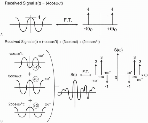 |
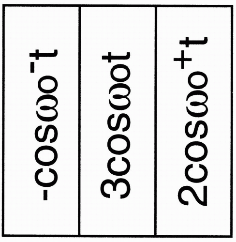 Figure 11-7. The sum of the signals in each column. Since the signals belonging to the same column have the same frequency, they are additive. |
Disadvantages
This technique is very dependent on external magnetic field inhomogeneities (i.e., it is sensitive to ΔB0).
This technique is also very sensitive to the magnetic field gradients. If the gradient is not perfect, you get artifacts.
Because of these disadvantages, this technique was given up.
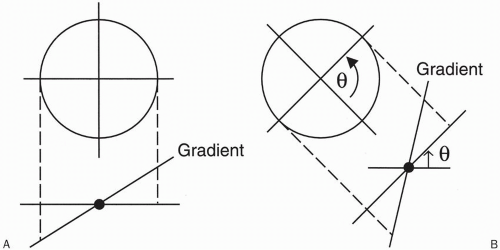 Figure 11-8. Back projection. By gradually rotating the gradient (from A to B
Get Clinical Tree app for offline access
Related posts:Stay updated, free articles. Join our Telegram channel
Full access? Get Clinical Tree


|