Pulse Sequences: Part I (Saturation, Partial Saturation, Inversion Recovery)
Introduction
A pulse sequence is a sequence of radio frequency (RF) pulses applied repeatedly during an MR study. Embedded in it are the TR and TE time parameters. It is related to a timing diagram or a pulse sequence diagram (PSD), which is discussed in Chapter 14. In this chapter, we discuss the concepts of saturation and consider pulse sequence partial saturation, saturation recovery, and inversion recovery (IR). In the next chapter, we’ll talk about the important spin-echo pulse sequence. Figure 7-1 illustrates the notations used for three types of RF pulses throughout this book.
Saturation
Immediately after the longitudinal magnetization has been flipped into the x-y plane by a 90° pulse, the system is said to be saturated. Application of a second 90° pulse at this moment will elicit no signal (like beating a dead horse). A few moments later, after some T1 recovery, the system is partially saturated. With complete T1 recovery to the plateau value, the system is unsaturated or fully magnetized. Should the longitudinal magnetization only be partially flipped into the x-y plane (i.e., flip angles less than 90°), then there is still a component of magnetization along the z-axis. The spins in this state are also partially saturated.
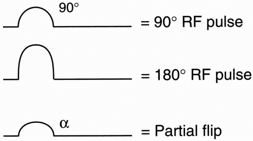 Figure 7-1. The notation for 90°, 180°, and partial flip pulses. |
Partial Saturation Pulse Sequence. Start with a 90° pulse, wait for a short period TR, and then apply another 90° pulse. Keep repeating this sequence. The measurements are obtained immediately after the 90° RF pulse. Therefore, the signal received is a free induction decay (FID).
Let’s see how this looks on the T1 recovery curve (Fig. 7-2). At time t = 0, flip the longitudinal magnetization 90° into the x-y plane. Right after that, the longitudinal magnetization begins to recover. Wait a time t = TR, and repeat the 90° pulse. Initially, at time t = 0, the longitudinal magnetization is at a maximum. As soon as we flip it, the longitudinal magnetization goes to zero and then immediately thereafter begins to grow. At time t = TR, the longitudinal magnetization has grown but has not recovered its plateau before it is flipped into the x-y plane again. (Note that the length of the longitudinal magnetization vector before the second 90° RF pulse is less than the original longitudinal magnetization vector.)
Now, with a third 90° RF pulse, we again flip the longitudinal magnetization into the x-y plane. Again, the longitudinal magnetization goes to zero and immediately begins to recover.
Again, at time 2TR, it is less than maximum but is equal to the previous longitudinal magnetization (at time TR). Each subsequent recovery time TR after each subsequent 90° pulse will also be the same. Thus, the maximum FID occurs at time t = 0 after the first 90° RF pulse, and all subsequent FIDs will have less magnitude but will have the same value.
Again, at time 2TR, it is less than maximum but is equal to the previous longitudinal magnetization (at time TR). Each subsequent recovery time TR after each subsequent 90° pulse will also be the same. Thus, the maximum FID occurs at time t = 0 after the first 90° RF pulse, and all subsequent FIDs will have less magnitude but will have the same value.
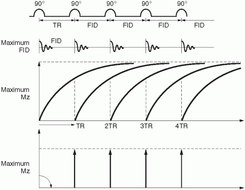 Figure 7-2. The recovery curves following the RF pulses in a partial saturation sequence. |
Question: Is there a residual transverse magnetization Mxy at time TR just before the next 90° RF pulse?
Answer: No! Because T1 is several times larger than T2, after a time TR has elapsed, the magnetization in the x-y plane has fully decayed to zero.
Answer: T1–weighted image.
A partial saturation pulse sequence generates a T1-weighted image.
Saturation Recovery Pulse Sequence
The previous sequence is called partial saturation because at the time of the second 90° RF pulse (at time TR), we haven’t yet completely recovered the longitudinal magnetization. Therefore, only a portion of the original longitudinal magnetization (M0) is flipped at time TR (and subsequent TRs). Hence the name partial saturation.
In saturation recovery, we try to recover all the longitudinal magnetization before we apply another 90° RF pulse. We have to wait a long time before we apply a second RF pulse. Thus, TR will be long (Fig. 7-3).
After each 90° RF pulse, we measure it and an FID right away. Because we allow the longitudinal magnetization to recover completely before the next 90° pulse, the FID gives the maximum signal each time. In other words, we have recovered from the state of saturation.
Answer: Proton density weighted (PDW).
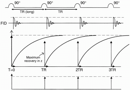 Figure 7-3. In a saturation recovery sequence, TR is long and longitudinal magnetization vectors are near maximal. |
The saturation recovery pulse sequence results in a proton density-weighted image.
Neither of these sequences is really used any more, but they are so simple to understand that they are good springboards from which to learn about other, more complex pulse sequences. These pulse sequences are not used because it is very difficult to measure the FID without a delay period. Electronically we have to wait a certain period of time to make the measurements. Also, external magnetic inhomogeneity becomes a problem; that’s why spin-echo sequences (which we will discuss in the next chapter) are used to eliminate this problem.
Inversion Recovery Pulse Sequence
In IR, we first apply a 180° RF pulse. Next, we wait a period of time (the inversion time TI) and apply a 90° RF pulse. Then we wait a period of time TR (from the initial 180° pulse) and apply another 180° RF pulse (Fig. 7-4), beginning the sequence all over again.
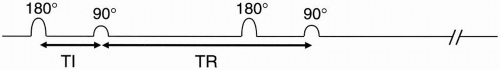 Figure 7-4. In inversion recovery, the time between the 180° pulse and the 90° pulse is denoted TI. |
Before we apply the 180° pulse, the magnetization vector points along the z-axis. Immediately after we apply the 180° pulse, the magnetization vector is flipped 180°; it is now pointing south (−z), which is the opposite direction (Fig. 7-5).
We then allow the magnetization vector to recover along a T1 growth curve. As it recovers, it gets smaller and smaller in the −z direction until it goes to zero, and then starts growing in the +z direction, ultimately recovering to the original longitudinal magnetization.
After a time TI, we apply a 90° pulse. This then flips the longitudinal magnetization into the x-y plane. The amount of magnetization flipped into the x-y plane will, of course, depend on the amount of longitudinal magnetization that has recovered during time TI after the original 180° RF pulse. We measure this flipped magnetization. Therefore, at this point we get an FID proportional to the longitudinal magnetization
flipped into the x-y plane. Also, at this point, we begin the regrowth of the longitudinal magnetization. Recall that for a typical T1 recovery curve, the formula for the exponential growth of the curve is 1 − e−t/T1 However, when the magnetization starts to recover from −M0 instead of zero (Fig. 7-6), the formula for recovery is 1 − 2e−t/T1
flipped into the x-y plane. Also, at this point, we begin the regrowth of the longitudinal magnetization. Recall that for a typical T1 recovery curve, the formula for the exponential growth of the curve is 1 − e−t/T1 However, when the magnetization starts to recover from −M0 instead of zero (Fig. 7-6), the formula for recovery is 1 − 2e−t/T1
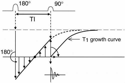 Figure 7-5. The recovery curves in inversion recovery. After the 180° pulse, the longitudinal magnetization vector is flipped 180° and starts to recover from a value that is the negative of its initial maximal value. |
Exercise
Verify the above formula mathematically.
Magnitude of signal intensity = − 1.
At t = ∞ (infinity), Signal intensity = 1 − 2e−∞/


Related posts:
Stay updated, free articles. Join our Telegram channel
Full access? Get Clinical Tree
