High Performance Gradients
Introduction
This chapter briefly discusses the new technology of high performance gradients. As you know by now, gradients have many purposes, including slice selection, spatial encoding, flow compensation (FC), and spoiling, rewinding, and presaturation. It should be fairly obvious that every time you use a gradient, you are lengthening the pulse cycle (thus increasing minimum TE).
Consider the two gradients in Figure 30-1A and 30-1B. The gradient in Figure 30-1A has half the strength of the one in Figure 30-1B but twice the duration. Thus, both these gradients have the same area (shaded area). They both achieve exactly the same result (e.g., phase shift) on stationary spins, but the second one is twice as fast and allows one to reduce the echo delay time TE. Therefore, the first requirement of a high performance gradient is a higher maximum strength.
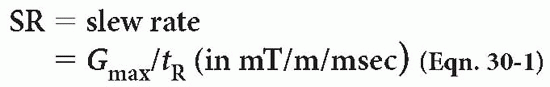
When we discuss high performance gradients, not only do we want to achieve a stronger magnitude or strength, but we also want the maximum strength to be achieved in as short a time as possible (i.e., a short rise time) to minimize the duration of the gradient. Therefore, the second issue is how fast a gradient can reach its plateau (Fig. 30-2). The ratio of the maximum gradient (Gmax) to the rise time (tR) is called the slew rate (SR).
Early gradients had a Gmax of 3 to 6 mT/m and a tR of 1.5 to 2 msec (i.e., SR of 1.5 to 4 mT/m/msec).
The requirements for high performance gradients are the following:
High gradient strength (Gmax)
Short rise time (tR)
i.e., a high slew rate (Gmax/tR).
In the mid-1980s, GE introduced shielded gradients with Gmax of 10 mT/m and tR of 675 µsec = 0.675 msec (i.e., SR of 15 mT/m/msec). The new high performance gradient systems (Siemens’ Sonata or Symphony with Quantum Gradients, GE‘s Twin Speed, Philips’ Intera, etc.) have Gmax as high as 40 mT/m and tR as low as 180 µsec with SR as high as 200 mT/m/msec .
Advantages
Shorter cycles are possible. As discussed previously, a stronger gradient can be applied over a shorter duration. Consider the example of FC. Figure 30-3 demonstrates two FC gradients that achieve the same thing, but the second one has higher strength (G′ > G) and is thus applied over a shorter period (T′ < T). (As an aside, because of the quadratic nature of phase accumulation for flowing spins, there is no linear or inverse linear relationship between gradient strength and application time, i.e., doubling the gradient strength does not halve the time of gradient application.) Higher order motion (e.g., acceleration, jerk) requires
the addition of even more gradient lobes. You can see how high performance gradients can save a lot of time during each cycle, allowing for shorter TEs (reducing dephasing) and TRs (for fast scanning).
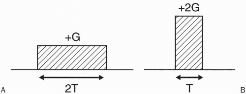
Figure 30-1. The gradient in (B) has twice the strength of the one in (A) but half the duration. Consequently, they both have exactly the same area and thus achieve the same results for stationary spins. However, the one in (B) has the advantage of being faster, a condition that is required for fast scanning.
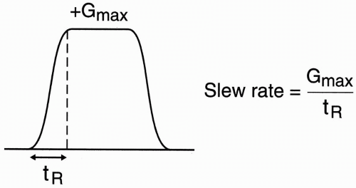
Figure 30-2. In reality, it takes a certain amount of time (tR) for a gradient to rise to its plateau Gmax. The ratio Gmax/tR is called the slew rate (in mT/m/msec).
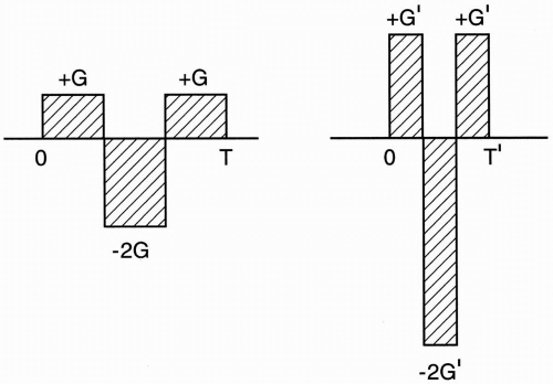
Figure 30-3. With high performance gradients, flow compensation can be accomplished faster (again because by increasing the strength and reducing the duration, the same area can be achieved).
Smaller field of views (FOVs) are possible. As we saw in Chapter 15, an inverse relationship exists between the gradient strength along one axis and the FOV: FOV = BW/(γG) where G is the gradient strength and BWRelated posts:

Stay updated, free articles. Join our Telegram channel

Full access? Get Clinical Tree