Signal Processing
Introduction
Signal processing refers to analog and/or digital manipulation of a signal. The signal could be an electric current or voltage, as is the case in magnetic resonance imaging (MRI). Image processing is a form of signal processing in which the manipulations are performed on a digitized image. Analog-to-digital conversion (ADC) is a process by which a time-varying (analog) signal is converted to a digitized form (i.e., a series of 0s and 1s) that can be recognized by a computer. An understanding of signal processing requires a basic understanding of the concept of frequency domain and Fourier transform (FT) because most of the “processing” of a signal is accomplished in the frequency domain and, at the end, the results are converted back into the time domain.
One of the key concepts in signal processing, as we shall see shortly, is the Nyquist sampling theorem. An understanding of the sampling procedure allows one to appreciate the relationship between the samples of a signal (in the time domain) and its bandwidth (in the frequency domain). Once this concept is grasped, the issue of aliasing (wraparound) artifact can be explained very easily. A knowledge of signal processing will also help the reader understand the more complicated, newer fast scanning pulse sequences presented in later chapters.
Sequence of Events
First, let’s summarize what has been discussed so far. Figure 12-1 illustrates a summary of a spin-echo pulse sequence. The following is a summary of the sequence of events:
As an aside, consider Figure 12-2. Plotting field strength versus position (Fig. 12-2), the gradient is represented as a sloped line. The slope of the line is a constant that we call G. The value y along this line with slope G at point x is y = Gx. This is a simple linear equation. Figure 12-2B plots gradient strength versus time. Figures 12-2A and 12-2B are used interchangeably to illustrate a linear gradient with strength G.
4. Right before we receive the echo, we apply a phase-encoding gradient (Gy). The symbol for the phase-encoding gradent is in Figure 12-3. This symbol denotes the multiple phase-encoding steps that are necessary as we cycle through the acquisition. Remember that one of the phaseencode steps may be performed without any gradient.
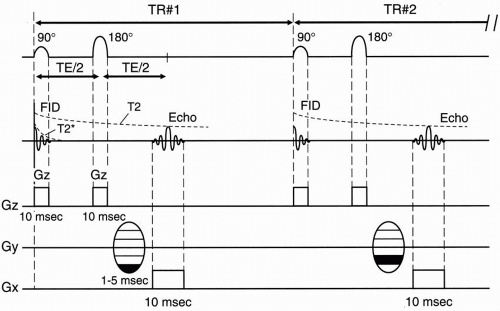 Figure 12-1. Spin-echo pulse sequence diagram. |
5. The frequency-encoding gradient (Gx) is turned on during the time period during which the echo is received.
6. Time requirements
The frequency-encoding step takes about 10 msec (4-8 msec at high field; 16-30 msec at lower fields).
The phase-encoding step takes 1-5 msec.
Then we repeat the whole sequence of events after time TR. The time spent from the center of the 90° pulse to the end of the echo readout is
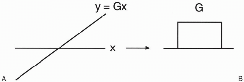 Figure 12-2. A linear G represents a linear function Gx, which can be represented either as a linear line with slope G (A) or as a rectangle with height G (B). |
The sampling time Ts is the time it takes to sample the echo, which is the time that the Gx gradient (readout or frequency-encode gradient) is on. The Gx gradient is on throughout the echo readout—from beginning to end (Fig. 12-4). The time from the beginning of the 90° pulse to the midpoint of the echo is TE. Because half of the sampling time continues past the midpoint of the echo, we need to add half the sampling time to TE to account for the entire “active time” from the beginning of the RF pulse to the end of the sampling time:
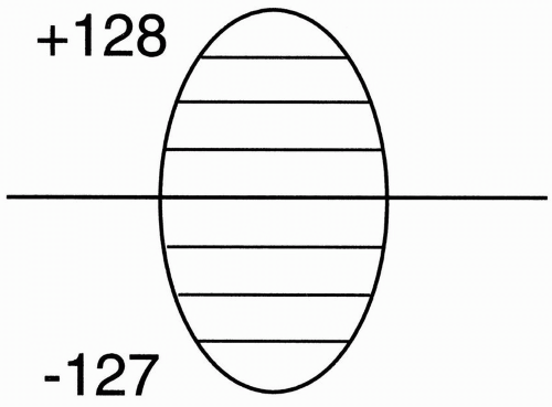 Figure 12-3. The symbol for phase-encode gradient. |
Active time = TE + Ts/2
There may also be time taken up by other events that occur before the RF pulse (such as presaturation pulses) that we include as overhead time (To). Thus,
Therefore, it takes 50 msec to read out the signal from one echo. We then place this signal into the data space (Fig. 12-5). We have designated 256 rows in the data space (from −127 to +128), and in this instance we’ve placed the first signal at position −127.
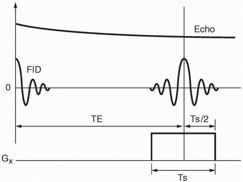 Figure 12-4. The frequency gradient is turned on during readout (i.e., during the echo). |
7. In the next TR cycle, we do exactly the same thing, except this time, the phaseencoding step will be done with a slightly weaker magnetic gradient and will be one step higher in k (data) space.
Question: Why does the magnitude of the signal differ with each phase-encoding step? For example, in Figure 12-5, the signal from the echo of TR#2 seems to have higher maximum amplitude than the signal from the echo of TR#1.
Answer: The strength of the phase-encoding gradient affects the magnitude of the signal.
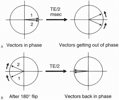
When the phase-encode gradient is at a maximum (when we have the largest magnetic field gradient), we have the maximum dephasing of proton spins. Recall that we are dealing with proton spins that have been flipped into the transverse plane by a 90° pulse, and the signal is maximum as long as these proton spins stay in phase. By using a magnetic field gradient, we are introducing an artificial external means of dephasing. Also, remember that when we flip the protons into the transverse plane, they are initially in phase and then rapidly go out of phase due to external magnetic inhomogeneities and spin-spin interactions (Fig. 12-6A). Next, the protons are flipped with a 180° pulse and, after a period of time = TE/2, they go back in phase (Fig. 12-6B).
On top of this, we introduce a magnetic inhomogeneity by way of a linear gradient in which the inhomogeneity increases linearly, causing additional dephasing of proton spins. We realize that we have to accept this additional dephasing because this is the way we obtain spatial information along the axis of this gradient. This process is called phase encoding.
However, this explains why, when we use the magnetic field gradient for phase encoding, the additional dephasing caused by the gradient will necessarily decrease the overall signal we receive during that phase-encoding step. It then allows us to conclude as follows:
The largest magnetic gradient we use for maximum phase encoding will give us the lowest magnitude signal.
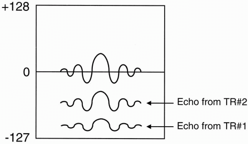
Figure 12-5. For each phase-encoding step, a signal is obtained that is placed in the data space.
When the magnetic gradient in the phaseencode direction is zero, we will not introduce any additional dephasing, and we will get the largest magnitude signal.
 |
k-space, as we mentioned in the last chapter (with more to come in Chapters 13 and 16), can
be thought of as a digitized version of the data space. The signal in the center of k-space (at position 0) has the maximum amplitude. This is because this signal is obtained at a phase-encoding step at which no magnetic field gradient is used (i.e., no phase gradient and hence no extra dephasing due to phase encoding). In fact, the center line of k-space will always be occupied by the phase-encoding step that uses no gradient.
be thought of as a digitized version of the data space. The signal in the center of k-space (at position 0) has the maximum amplitude. This is because this signal is obtained at a phase-encoding step at which no magnetic field gradient is used (i.e., no phase gradient and hence no extra dephasing due to phase encoding). In fact, the center line of k-space will always be occupied by the phase-encoding step that uses no gradient.
The center line of k-space will always contain the phase-encoding step with the weakest gradient and thus with the most signal.
The most peripheral lines of k-space will be occupied by the phase-encoding steps that use the strongest gradients.
The periphery of k-space will contain the phase-encoding steps with the largest gradients and thus with the least signal.
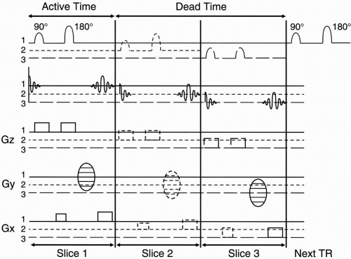 Figure 12-7. Multislice acquisition. During each TR cycle, there is a certain “dead time” that can be used to acquire other slices. |
8. Multislice technique
Remember that TR is much longer than the active time needed to perform all the functions necessary to select a slice, phase encode, and frequency encode. The TR might be, say, 1000 msec. The active time in our example was 50 msec. There is a lot of “dead time” in between the 50 msec of active time and the next 90° pulse. We can take advantage of this “dead time” in order to get information regarding other slices.
As an example, in Figure 12-7 we will have time for two additional slices to be studied during the dead time within one TR period. After we obtain the signal from slice number 1, we can apply another 90° pulse of a different center frequency ω, but with an identical transmit bandwidth to specify the next slice (Fig. 12-8). Here we are talking about the transmitted bandwidth (of the RF pulse) that determines slice thickness, not to be confused with the receiver bandwidth (of the echo) that determines noise. More on this later.
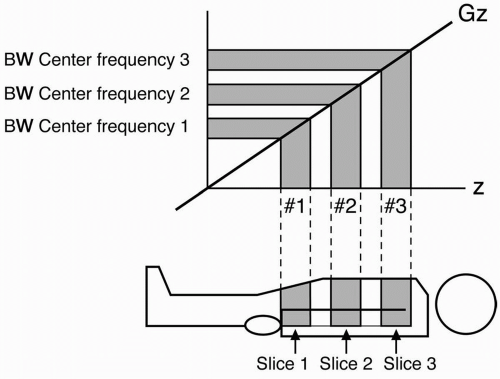 |
To choose the next slice, we keep the same magnetic gradient Gz, but we choose a bandwidth at a higher or lower center (or Larmor) frequency to flip the protons 90° in a different slice. The bandwidth is the same as the first slice, but the center frequency is different.
We choose the same phase-encoding gradient Gy so we get the same amount of dephasing in this next slice. We sample the echo with the same frequency-encoding gradient as we did with the first slice. Because we still have time during the dead time to acquire a third slice, we repeat everything and again choose a 90° RF pulse of a different Larmor frequency so we can flip the protons of a different slice into the transverse plane. The signal from each slice will be placed in a different k-space.
Each slice has its own k-space.
Slice selection can be performed in several different ways. We can have contiguous slices; sequential slices with a gap between slices; and interleaved slices, where we do odd-numbered slices (i.e., 1, 3, 5) and then go back and do evennumbered slices (i.e., 2, 4, 6).
9. Number of slices (coverage)
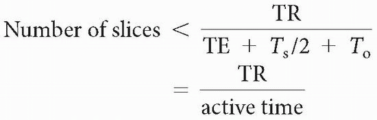
The number of slices we can do within any TR is limited by the dead time after (TE + Ts/2 + To). Furthermore, if we choose to have two echoes per TR (as in a dual-echo, spin-echo sequence), the number of slices we could have would be cut back more. The formula for the maximum number of slices one can obtain is
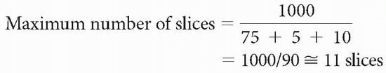
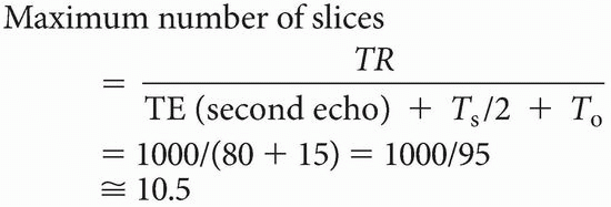
If we do multiple echoes (or just one long echo), the formula is governed by the longest TE.
Examples
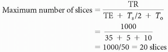
We usually don’t know what the sampling time (Ts) or overhead time (To) is; therefore, a rough approximation is
It is said that in a double-echo sequence, the first echo is “free.” This means that the number of slices in a double-echo sequence is determined only by the TE of the second echo
Maximum number of slices
In fact, the maximum number of slices is determined by TR, and the time it takes to get one line in the data space as follows:
Maximum number of slices < TR/time to get one line of signal into the data space = TR/(TE + Ts/2 + To)
Also remember that each slice has its own data space (and, thus, its own k-space), and if we are doing a double-echo sequence, each echo has its own data space (k-space). The signal obtained from each slice during the same TR will be obtained with the same phase-encoding step. Thus, the equivalent line in each data space of the slices for a given TR will be subject to the same dephasing effects of the phase-encoding gradient (Fig. 12-9).
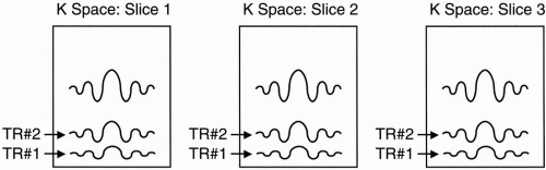 Figure 12-9. Each slice has its own k (data) space. |
Related posts:
Stay updated, free articles. Join our Telegram channel

Full access? Get Clinical Tree


