(1)
MGH Department of Radiology, Harvard Medical School, Newton, MA, USA
Abstract
Figure III.1 teaches us a little lesson: it’s not about what you look at, it’s all about what you see. From this point of view, an acquired image is nothing but a huge dataset, which still needs to be fed to your visual sensors, transmitted to your neurons, and processed with the latest version of your brain’s firmware. No wonder we need to repackage the imaging data so that it reaches our brains in the most meaningful way. This section will help us understand the mechanics of repackaging.
Key Points
The range of medical image intensities typically exceeds that of commercial displays. This creates a need for various intensity transformations, from plain contrast/brightness enhancements to complex nonlinear intensity rebalancing, which can help explore the rich contents of imaging data.
It is not about what you look at, it’s all about what you see. From this point of view, an acquired image is nothing but a huge dataset, which still needs to be fed to your visual sensors, transmitted to your neurons, and processed with the latest version of your brain’s firmware. No wonder we need to repackage the imaging data so that it reaches our brains in the most meaningful way. This section will help us understand the mechanics of repackaging.
7.1 From Window/Level to Gamma
Let me assume, my dear reader, that you are somewhat familiar with the concept of Window/Level (W/L), briefly mentioned before. Also known as brightness/contrast adjustment,1 W/L helps us zoom into various ranges of image intensities that typically correspond to different tissues and organs. You can find W/L in virtually any medical imaging application, not to mention the remote control of your TV set.
W/L has one important property: it is linear. This means that it maps a selected subrange of the original image intensities [i 0,i 1] into the full [0,M] range of display luminance, using a straight-line function (Fig. 7.1). That’s what makes it so similar to zoom: in essence, W/L magnifies all [i 0,i 1] intensities by a constant  factor, so that they can span the entire range of monitor luminance. All intensities below i 0 are truncated to 0, and above i 1 – to M.
factor, so that they can span the entire range of monitor luminance. All intensities below i 0 are truncated to 0, and above i 1 – to M.Fig. 7.1
Window/Level function displays a selected range of the original image intensities [i 0 , i 1]
W/L is probably the most frequently used button on your diagnostic workstation toolbar, and it does a wonderful job of localizing different organs and tissues (Fig. 7.2). W/L is also the only practical way to explore the full intensity spectrum of 16-bit DICOM images, using that plain 8-bit monitor sitting on your desktop. As we pointed out earlier, 16-bit medical images can contain up to 216 = 65,536 shades of gray, while plain consumer monitors can show only 28 = 256 of them at once. Clearly, 65,536 does not fit into 256, but W/L solves this problem, enabling us to browse through the original 65,536 shades, displaying only the intensities that matter to us at any particular moment – such as [i 0 ,i 1] range in Fig. 7.1. Without W/L, we would have to depend on more complex and considerably more expensive monitor hardware capable of displaying deeper than 8-bit grayscale – hardware that may be hard to find and install. In essence, it was the W/L function that contributed to the proliferation of teleradiology, smartphones, tablets and web viewers, to reach far beyond the grasp of your bulky PACS workstation.
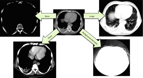
Fig. 7.2
Use of linear W/L transform to select different [i 0,i 1] intensity ranges in CT image. Note that the image includes everything from diagnostic tissues to pure noise
In short, we should all bow and thank W/L for being so useful and handy. But you, my inquisitive reader, would certainly like to go beyond the basics, wouldn’t you? So what if we consider nonlinear, curved mapping? Look at Fig. 7.3: unlike the “bone” example in Fig. 7.2, this transform improves the original bone contrast, but you can still see the soft tissues. This suggests a nonlinear function f LUT (i), which cannot be expressed as a fixed-factor intensity zoom. Instead, it amplifies different intensities with different factors – less for darker, and more for brighter. If we want to keep our zoom analogy, this is similar to the fish eye effect.
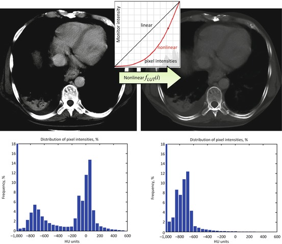
Fig. 7.3
Nonlinear intensity transformation. Unlike W/L, which merely selects intensity subranges, nonlinear transforms change the distribution of pixel intensities. The graphs under the images show their histograms – plots of pixel value frequencies. Note how bright intensities centered around zero HU on the left histogram disappeared – they were moved into the darker intensity ranges of negative HUs
For example, consider  for some constant value γ > 0. This power transform is known as gamma correction. When γ = 1, it is linear
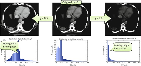
  , which is identical to a W/L transform with W = 2 × L = i max . However, the more different γ becomes from 1, the more nonlinearly f γ (i) behaves – check out Fig. 7.4, which illustrates the differences in f γ (i) for γ = 0.5 Wnd γ = 2.0. You can see that f γ = 0.5(i) amplifies lower (darker) intensities at the expense of suppressing the higher (brighter) ones. Therefore for 0 < γ < 1, it is often called “dark enhancement”, as it improves the visibility (contrast) for the dark image shades. For the same reason, γ > 1 provides “bright enhancement”.
for some constant value γ > 0. This power transform is known as gamma correction. When γ = 1, it is linear , which is identical to a W/L transform with W = 2 × L = i max . However, the more different γ becomes from 1, the more nonlinearly f γ (i) behaves – check out Fig. 7.4, which illustrates the differences in f γ (i) for γ = 0.5 Wnd γ = 2.0. You can see that f γ = 0.5(i) amplifies lower (darker) intensities at the expense of suppressing the higher (brighter) ones. Therefore for 0 < γ < 1, it is often called “dark enhancement”, as it improves the visibility (contrast) for the dark image shades. For the same reason, γ > 1 provides “bright enhancement”.Fig. 7.4
Gamma correction, applied to the [0, 600] range of the original pixel values (expressed in CT HU units)
What is particularly interesting is that the “dark vs. bright” rebalancing helps gamma correction to undo some of the HVS artifacts. Our visual system works better in the dark: humans see more contrast in dark shades than they do in bright ones. This helped our little furry prehistoric ancestors hunt and survive at night. For that reason, if we want to see as objectively as digital cameras and medical scanners do, we need to compensate for this “night-day” nonuniformity. This can be done if we pack more image shades into the dark part of the luminance spectrum – the part where we can see better, and therefore can see more. But this is exactly what gamma correction does for γ > 1 – it moves more image shades into the darker luminance spectrum (Fig. 7.4, right). Thus, we arrive at our first attempt to achieve HVS-neutral image display, with nothing but a simple γ > 1 power transform.
This ability to make shades more visible is one of the reasons that gamma correction became popular with graphics hardware manufacturers. Many displays would be preconfigured to use γ around 2.2 to make the images more vivid – that is, packing more shades into our favorite dark-intensity zone. This luminance arrangement also enables us to differentiate among more similar shades. Make a mental note here – we will revisit the “more shades” approach and magic γ > 1 a bit later, when we talk about DICOM calibration.
Finally, from the implementation point of view, nonlinear intensity transforms lead to an interesting concept of Look-Up Tables (LUT) – a concept that profoundly affects the ways we look at the images. The problem is that nonlinear functions like f LUT (i) can be quite complex. In fact, they may not even have easy formula-like expressions. Recomputing f LUT (i) every time and for every pixel would simply kill any image-processing application. This is why the simplest way to store and apply nonlinear transforms is to keep them in tables: for each original image intensity i we define the corresponding display luminance m i = f LUT (i). Then once m i are stored in the LUT, we read them from there instead of recomputing f LUT (i) values again. Think about using some LUT transform while scrolling through a long stack of MR images: every pixel in every image will have to be transformed with f LUT () before it is thrown on the screen. This is exactly the case when calling f LUT () for all pixels will take forever, but fetching m i = f LUT (i) from the LUT table – a few instants.
Nota bene:
Without a doubt, you can also use LUT to tabulate the linear W/L function f WL (i). But when it comes to hardware implementation, linear transforms can usually be defined and applied directly, without the need for any LUT; besides, not using LUT saves memory. Complex nonlinear transforms, on the contrary, need LUT format to be stored in computer memory. This does imply certain memory overhead, but we do not have to compute complex transform values every time we need them. Thus, we gain performance.
7.2 Histogram Equalization
Related posts:
Stay updated, free articles. Join our Telegram channel

Full access? Get Clinical Tree


