Image Enhancement

(1)

MGH Department of Radiology, Harvard Medical School, Newton, MA, USA

Abstract

Physicians don’t like image-enhancing functions because they do not trust them. And they have all the reasons to be skeptical. For a good deal of this book we’ve been playing the same tune: digital data is rigid, and once acquired, it cannot be perfected with more information than it had originally. How, then, can this pixel matrix, so static and invariable, be made any better? Where the enhancements could come from?

I am a man of simple tastes easily satisfied with the best

Winston Churchill

Key Points

Once a digital image is acquired, nothing else can be added to it – the image merely keeps the data it has. Nevertheless, different components of this data may have different diagnostic meaning and value. Digital image enhancement techniques can emphasize the diagnostically-important details while suppressing the irrelevant (noise, blur, uneven contrast, motion, and other artifacts).

The answer is intriguingly simple: they won’t come from anywhere. They are already in the image, hidden under the clutter of less important and diagnostically insignificant features. We simply cannot see them, yet they do exist in the deep shades of DICOM pixels. This is why any image enhancement technique – from basic window/level to very elaborate nonlinear filtering – is nothing but an attempt to amplify these most important features while suppressing the least diagnostic. Simply stated, it is sheer improvement of visibility of the already present diagnostic content.

This sounds reasonable and easy, but as always, the devil is in the details… To put this puzzle together, we’ll do a little case study, departing from the less practical basics, and arriving at something that can actually be used.

5.1 Enemy Number One

Noise is the major enemy of any meaningful image interpretation. Noise is also the most common artifact, inevitably present in every natural object, process, or data – including images. Noise can be purely random (such as “white” noise in X-rays) or more convolved (such as “reconstructed” streak-like noise in CT images) – but if it does not contain diagnostic information, it is useless and destructive. Can it be removed?

Yes, with a certain degree of success, and with a certain artistry of peeling the noise from the noise-free data. To do so, we have to look at it through computer eyes first. Consider Fig. 5.1; it shows a small 3 × 3 pixel matrix sample with nine pixels p _i, taken from a real image. Do you see noise?

Fig. 5.1

Small 3 × 3 pixel sample with noise

Well, the pixel values p _iare definitely non-constant and fluctuate somewhere around the 100 average. But it is the center pixel p ₀ = 65 that really falls out, way too low compared to the surrounding values. Certainly, one may argue that p ₀is depicting some real phenomenon: small blood vessel section, microcalcification, or anything else. But in most cases we expect all diagnostic phenomena to take more than a single pixel (the entire premise behind ever-increasing medical image resolution); one cannot build a sound diagnosis on a single dot. This reasoning brings us to a more “digital” definition of the image noise: abrupt changes in individual pixel values, different from the surrounding pixel distribution.

This means that the only way to remove p ₀’s noise is to use the neighboring pixels. There are several simple techniques traditionally mentioned when one starts talking about fixing the noisy data. Figure 5.2 shows the most classical one: linear (aka low-pass, Gaussian) smoothing filter. It replaces each pixel p ₀ by a new value q ₀, computed as a w _i-weighted average of all p ₀’s neighbors¹ (Eq. 5.1). The positive constants w _iare usually borrowed from bivariate Gaussian distribution:

Fig. 5.2

Gaussian denoising. Weights w _i(center) were sampled from bivariate Gaussian distribution and normalized to have a unit sum (Eq. 5.1). Summing up p _ivalues multiplied by their respective w _iproduced a filtered pixel value p ₀ = 78

$\begin{array}{l}{q}_0={\displaystyle \sum_{0\le i\le 8}{w}_i{p}_i},\\ {}{w}_i= const\ge 0,\kern1em {\displaystyle \sum_{0\le i\le 8}{w}_i}=1\end{array}$

(5.1)

Averaging is quite simple and intuitive, and if you think about it a bit more, you might realize that it closely relates to both image interpolation (recovering the missing p ₀value with linear interpolation in Eq. (5.1)) and compression (predicting p ₀from its neighbors) – the techniques we discussed in the first part of this book. Yet now we are trying to pitch the same method for removing the noise – should it solve all our problems?

It shouldn’t, but in many cases natural noise consists of equally probable negative and positive oscillations jumping around a zero mean. So when we average the pixel values, negative and positive noise instances cancel each other, leaving us with the pure, noise-free pixels. It’s reasonable, it’s simple, it’s easy to compute – in short, it’s too good to be true.

Look at Fig. 5.3: averaging leads to smoothing of the image. It reduces the noise at the expense of making the entire image fuzzier.² This is why smoothing is useful for extracting large image features, but not for improving diagnostic quality – Gaussian filtering is also commonly referred to as Gaussian blur, and blurring is the last thing we want in image enhancement. This makes Gaussian filters, so abundant in imaging apps, fairly useless for our clinical needs; although good in theory, they fail to provide a decent diagnostic output.

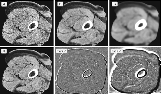
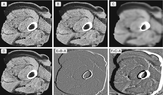
Fig. 5.3

Gaussian denoising filter, applied to the original noisy image A. Image B shows the result of a single Gaussian filtering, and image E shows the difference between B and A. Image C is the result of ten Gaussian iterations (and F = C − A) – as you can see, more Gaussian filtering produces even more blur. Image D shows a better original image, initially acquired with less noise. In theory, we want the filtered A to approach D, but Gaussian filtering in B and C loses all sharp image details

Nota bene:

The outcomes of imaging filters may be very subtle – can you always spot filter-related artifacts?

You can, and there are two practical ways to see what you gained and what you lost with any particular filter:

Apply the filter several times. As we learned from the previous sections and Fig. 3.3 C, this will accumulate filter artifacts, making them crystal-clear.

Compute a difference image, subtracting original image from the filtered. The difference will show exactly what the image has lost after the filtering.

We can learn from our little Gaussian fiasco and consider another example of a basic, yet non-Gaussian noise removal approach. Known as a median filter, it attempts to fix the blurring problem by using pixel median instead of pixel average:

${q}_0=\underset{0\le i\le 8}{\mathrm{median}\ }\left\{{p}_i\right\}$

(5.2)

– that is, replacing p ₀ by the central value from the sorted pixel sequence (Fig. 5.4).³

Fig. 5.4

Median filter replaces p ₀ with the median value from the {p ₀,…,p ₈} sequence. Medians are less dependent on the outliers, and will not blur the edges

You would probably agree that median-filtered image B in Fig. 5.5 does look better and sharper than its Gaussian-filtered counterpart B in Fig. 5.3. It’s true, and median filters can do a pretty decent job removing “salt and pepper” noise – isolated corrupted pixels, surrounded by noise-free neighbors. But this is a rather idealized scenario, hard to find in real clinical data, where neighbors of the noisy pixel will be noisy as well, and so will their medians. Besides, instead of Gaussian blur, the median filter suffers from intensity clustering, exemplified in Fig. 5.5C – when several pixel neighbors start forming same-intensity blobs. This clustering destroys the natural image texture even at a single filter pass – which cannot be accepted in diagnostic denoising.

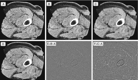
Fig. 5.5

Median filter, and the same imaging experiment: noisy original A, filtered with one (B) and ten (C) passes of the median filter. Image E = B − A and image F = C − A. Image D is a noise-free original that we would like to approach with B. Unlike the Gaussian filter, the median filter does not blur, which is why it removes mostly noise and does not touch the structural elements (difference image E shows mostly random noise). However, the median filter tends to grow clusters of same-color pixels – this is somewhat visible in B, and very apparent in C, with its brushstroke-like pattern. This clustering destroys the natural texture of the image, and although we still remove the speckled noise, the filtered images look far from the ideal D

Nonetheless, the median filter introduces us to the next level of nonlinear filtering, which cannot be done with w _i-weighted pixel averaging, used by Gaussian and the like. Nonlinearity proves to be a really fruitful concept, leading to more sophisticated processing, capable of real medical image enhancement. The bilateral filter is one of the most popular of the nonlinear breed (Tomasi and Manduchi 1998; Giraldo et al. 2009). To fix the Gaussian approach, the bilateral filter redefines the weights w _ito become non-constant functions of pixel intensities and distances (Eq. 5.3):

$$$ \begin{array}{c}{q}_0=\frac{p_0+\lambda {\displaystyle \sum_{j\ne 0}{w}_j{p}_j}}{1+\lambda {\displaystyle \sum_{j\ne 0}{w}_j{p}_j}},\\ {}{w}_j={e}^{-{\left(\frac{p{}_0-{p}_j}{\sigma_v}\right)}^2}{e}^{-{\left(\frac{\left\Vert p{}_0,{p}_j\right\Vert }{\sigma_d}\right)}^2},\kern1em \\ {}\left\Vert p{}_0,{p}_j\right\Vert =\sqrt{{\left({x}_{p_0}-{x}_{p_1}\right)}^2+{\left({y}_{p_0}-{y}_{p_1}\right)}^2}\kern0.24em \\ {}\kern0.6em -\mathrm{distance}\;\mathrm{between}\;\mathrm{pixel}\;{p}_j\;\mathrm{and}\;\mathrm{center}\;\mathrm{pixel}\;{p}_0,\\ {}\lambda, {\sigma}_v,{\sigma}_d= const>0\kern1.32em -\mathrm{filter}\;\mathrm{parameters}\\ {}{e}^x= \exp (x)\kern0.48em -\mathrm{exponent}\;\mathrm{function}\end{array} $$ ” src=”/wp-content/uploads/2016/03/A317927_1_En_5_Chapter_Equ3.gif”></DIV></DIV><br /> <DIV class=EquationNumber>(5.3)</DIV></DIV></DIV><br /> <DIV class=Para>The equation for <SPAN class=EmphasisTypeItalic>w</SPAN> <SUB><SPAN class=EmphasisTypeItalic>j</SPAN> </SUB>may look somewhat complex to an unprepared eye, but it has a very simple interpretation: weighting coefficients <SPAN class=EmphasisTypeItalic>w</SPAN> <SUB><SPAN class=EmphasisTypeItalic>j</SPAN> </SUB>are made to be high when two pixels <SPAN class=EmphasisTypeItalic>p</SPAN> <SUB>0</SUB> and <SPAN class=EmphasisTypeItalic>p</SPAN> <SUB><SPAN class=EmphasisTypeItalic>j</SPAN> </SUB>are close in both location and intensity (Fig. <SPAN class=InternalRef><A href=$ 5.6). In this way, weight w _jdefines pixel similarity, and neighbors most similar to the central p ₀ receive the highest weights. Thus, instead of simply averaging the p _jvalues with the Gaussian filter, the bilateral filter replaces p ₀ with the average of its most similar neighbors.

Fig. 5.6

Left: Here is how bilateral filter coefficient w _jdepends on the proximity between p ₀ and p _j, both in pixel intensity and location. When p ₀ and p _jbecome close (differences in their location and intensity approach 0), w _jreaches its maximum, indicating that both pixels are similar and can be used to correct each other’s values. Otherwise, w _jbecomes negligibly small, meaning that dissimilar p _jshould not contribute in the filtered value of p ₀. Right: The neighbors p _jsimilar to p ₀ will have higher weights w _j, thus contributing more to denoising of the p ₀ value

It’s easy to understand why this approach can remove noise while being gentler on the local details and edges:

If p ₀ intensity is significantly different from the surrounding p _j, then w _jwill be nearly-equally low, and p ₀ will be replaced by an average of its neighborhood. This is the case of the Gaussian filter’s removal of a stand-alone noisy pixel; higher values of λ will produce a higher degree of averaging.

Otherwise, if p ₀ has a few similar pixels around, their weights w _jwill prevail in (Eq. 5.3), making the other terms negligible. As a result, the value of p ₀ will be adjusted to the average of its most similar neighbors, producing a rather small p ₀ change. This is the case of preserving a local image detail, formed by several similar pixels. Thus, the bilateral filter will not make the details fuzzy.

As Fig. 5.7 suggests, bilateral filtering can do a pretty good job in image denoising: it avoids indiscriminate Gaussian blur, and escapes median filter brushstrokes. This makes the bilateral filter a good practical choice for diagnostic image denoising applications, and I would recommend having it on your filter list.

Fig. 5.7

Bilateral filter. In essence, the bilateral filter (single iteration in B, and ten iterations in C) can be viewed as an “edge-aware” Gaussian: it smoothes only similar pixels. Therefore the result of its application B approaches ideal noise-free original D. The choice of the filter parameters (λ, σ _v, σ _d

Only gold members can continue reading. Log In or Register to continue