Intravoxel Incoherent Motion and Non-Gaussian Diffusion-Weighted Imaging: Introduction
The role of breast magnetic resonance imaging (MRI) has expanded into many clinical applications, including differentiation between benign and malignant breast lesions, preoperative staging, evaluation of high-risk patients, and implant assessment. For breast diffusion-weighted imaging (DWI), as described in the previous chapters, apparent diffusion coefficient (ADC) has been well investigated for differentiating malignant and benign breast tumors, although not yet incorporated into the Breast Imaging Reporting and Data System (BI-RADS) classification. ADC, calculated using the monoexponential Gaussian model, has been utilized mainly for breast tumor characterization and has revealed various meaningful results. ADC values in breast cancer often are lower than benign tumors or normal breast tissue, and international efforts are underway toward implementing diagnostic ADC thresholds and standardizing the acquisition protocol of breast DWI.
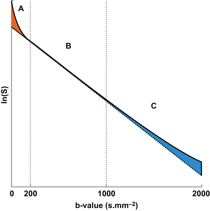
It is also known that the DWI signal contains more information to be extracted and clinically utilized. In terms of signal intensity, at low b values (around ≤200 s/mm 2 ) the decay of measured signal attenuation in vivo is faster than at intermediate b values, whereas it is slower at larger b values (at least ≥1500 s/mm 2 ; Fig. 8.1 ). Consequently, non-Gaussian diffusion models are proposed to better describe diffusion signal behavior, which can have a direct link with tissue physiological and pathological characteristics. Signal behavior at low/intermediate values is often characterized by the intravoxel incoherent motion (IVIM) model, whereas departures from exponential signal decay at high b values are treated with various descriptions broadly termed non-Gaussian DWI. Non-Gaussian descriptors therefore attempt to move beyond this most simple concept of diffusion, toward a more accurate view of the underlying processes. Interpretation of observed non-Gaussian diffusion in vivo therefore requires a closer look at the process and properties of water molecule motion within tissue and an understanding of the mechanisms of image and contrast formation in DWI.
With the increasing use of the IVIM model in clinical research, throughout the body and including the breast, the interest in more complex and extended descriptions of diffusion has become commensurately greater. Although the IVIM model has generated a great deal of interest and has been the subject of much research, it is not without its challenges. With the advent of high performance gradient hardware systems in clinical MRI scanners, the access to high b values (beyond 1000 s/mm 2 ) has triggered interest in more complex and extended descriptions of diffusion beyond the standard ADC to supply new and useful information on tissue microstructure.
DWI has relatively lower sensitivity compared with dynamic contrast-enhanced (DCE) MRI, and improved diagnostic performance using a multiparametric approach combining DWI and DCE MRI has been reported by several groups. Still, although DCE MRI is a gold standard and the core of breast MRI, it requires the injection of gadolinium-based contrast agent, which is problematic for some with counterindications. Thus another benefit of IVIM and non-Gaussian DWI is that it can provide quantitative information on microcirculation and microstructure in tissues without the use of contrast agents.
This chapter introduces the methods and clinical application of IVIM and non-Gaussian DWI in the breast. First, fundamentals of Gaussian and non-Gaussian diffusion are reviewed, along with their common manifestation in clinical MRI (e.g., IVIM, diffusion kurtosis imaging [DKI]). Next, the literature of clinical applications of IVIM and non-Gaussian DWI in breast cancer is reviewed, including malignancy determination, prognostic factor correlation, and treatment response prediction. Then, methods of image acquisition of advanced breast DWI are reviewed, followed by discussion of data analysis strategies ( b value choices, fitting algorithms, model comparison, and noise handling). Finally, a brief discussion is provided on the balance between microstructural characterization and clinical value, as well as the potential for wide-scale translation of IVIM and non-Gaussian DWI in the breast.
Diffusion in Tissue: Fundamentals
The term Gaussian relates to the distribution of the diffusion-driven molecular displacements in a free medium without borders (see Fig. 1.1 ), as in a glass of water or the cystic component of a lesion. This is also known as Brownian motion, “free” or “true” diffusion, in which any water molecule is free to randomly move in any direction without limit. Gaussian relates to the normal shape of the diffusion propagator , a mathematical description of the probability of finding a water molecule at a specific point away from its original position after a given time ( Fig. 8.2 ). In bulk fluids, the Gaussian diffusion coefficient is then linked to the intrinsic properties of the diffusing molecule (mass, size) and the medium (viscosity). This diffusion coefficient is independent of the choice of b values. However, in biological tissues molecular diffusion is hindered by many obstacles (e.g., cell membranes, blood vessels, fibrosis). As a result, diffusion displacements get shorter and the distribution of molecular displacement is no longer Gaussian (see Fig. 1.1 ). Hence diffusion coefficients, though still analyzed with a Gaussian model, are referred to as apparent diffusion coefficients.

Beyond the notion of restricted but Gaussian-appearing diffusion characterized by a single ADC, there are observable deviations from Gaussian behavior both at low b values and high b values. These two regimes are discussed separately later. Within this topic, the distinction between a biophysical model of a system and a purely mathematical representation is important; and we will see that some non-Gaussian descriptions are quite clearly of this latter form, and we do not attempt to explicitly describe or quantify microstructure. Two goals of performing breast DWI predominate: (1) characterization of the underlying physiology/microstructure and (2) generating biomarkers for patient management. These goals often align and are synergistic but must be appropriately prioritized. The microstructure of the breast is quite complex (comprising fibroglandular tissue [FGT] with stroma and lobular/ductal structures, adipose tissue, microvasculature, as well as possible malignant epithelium or benign hyperplasia, cysts, fibrosis, or other growths), and inferring all details of this mixture can be limited by the available data and by intravoxel heterogeneity. It is therefore pragmatic to assume that any successful description of the diffusion decay curve will be at least somewhat empirical. With this in mind, we proceed to discuss IVIM and non-Gaussian DWI contrast in general and for the particular case of breast tissue.
Intravoxel Incoherent Motion (IVIM)
The biophysical model of IVIM is that the DW signal originates from two compartments: molecular diffusion in tissues and microcirculation (perfusion). This is based on the assumption that the flow of blood through capillaries mimics a diffusion process due to the pseudorandom organization of capillaries in tissue. To separate the effects of diffusion and perfusion on the DW signal, a biexponential model can be formulated as follows:
S(b)/So=fexp(−b(Dblood+D*))+(1−f)exp(−bD)
where f is the flowing blood fraction, D * is the pseudodiffusion coefficient associated with blood microcirculation, D blood is the water diffusion coefficient in blood (a term often omitted or absorbed into D * in practice), and D is the apparent diffusion coefficient in the tissue space. In most cases, the pseudodiffusion coefficient associated with blood microcirculation is much larger (about 10 times larger) than the water diffusion coefficient in tissues. As depicted in Fig. 8.1 , the initial slope of the diffusion decay signal observed at low b values ( b < 200 s/mm 2 ) contains a mixture of perfusion and diffusion effects, whereas diffusion effects dominate at higher b values (200 < b < 1000 s/mm 2 ). Appropriate b value ranges for IVIM analysis are described in more detail later and depicted in Fig. 8.1 as regimes A and B.
f is sometimes called “ f IVIM ” or “ f p ,” D * is sometimes referred to as “ D p ,” “ ADC fast ,” or “ ADC high ,” whereas D is sometimes called “ D t ,” “ ADC slow ,” or “ ADC low ,” not to be confused with the standard ADC , whose calculation includes both perfusion-related and genuine diffusion effects. Regardless of nomenclature, the basic interpretation of the IVIM parameters are that (1) D reflects microstructure of the extravascular space from restricted/hindered diffusion, including cancerous cellularity; (2) f represents a blood volume marker; and (3) D * reflects a combination of blood velocity and vascular architecture. Here we employ the ( D, f, D *) notation when summarizing the literature for consistency.
Although the biexponential model ( Eq. 1 ) is the most commonly used form of IVIM analysis, it should be noted that it reflects only one scenario of the general case. Namely, pseudodiffusive behavior occurs in the long time limit of spins undergoing many directional changes over the echo time. In the opposite, short-time limit (also known as ballistic regime ), where spins largely reside in one capillary segment, the signal behavior is described by a sinc-function expression. In the intermediate case, an admixture of behaviors occurs that can be teased apart with advanced methods of flow compensation and time-dependent IVIM that are beyond the scope of this chapter. But from a fundamental point of view, the approximate nature of the common biexponential description should be kept in mind.
Non-Gaussian Dwi
From an empirical perspective, anything that gives rise to a diffusion signal decay as a function of the diffusion-weighting b value that deviates from a monoexponential form can be defined as non-Gaussian. This definition encompasses a variety of microstructural features, from a single restricted compartment to differently hindered compartments to multiply sized compartments; this empirical point of view leads to the creation and formulation of mathematical descriptions that are able to describe the observed decay curves. In this chapter we will review non-Gaussian MRI techniques that have been applied in breast tissue and breast cancer. Furthermore, we categorize them in two groups: those that sample non-Gaussianity as a function of diffusion weighting strength ( b value) and those that sample non-Gaussianity as a function of diffusion time.
Non-Gaussianity in Spatial Scale: b value Dependence
Acquisition and analysis using DW images at high diffusion weighting ( b ~ 1000–2000 s/mm 2 ) allow capturing such diffusion behavior beyond a single Gaussian diffusivity. A detailed description of the mathematics of every non-Gaussian approach is outside the scope of this chapter, and so later sections will focus on an illustrative few as applied to breast DWI, and discussing some of the related literature results. These techniques vary the b value as the primary contrast variable.
Diffusion Kurtosis Imaging
Diffusion kurtosis imaging (DKI), first developed by Jensen and colleagues, is a mathematical representation using an extended b value range that captures the nonmonoexponential (non-Gaussian) nature of the signal decay curve at high b values. DKI includes an additional parameter K , known as the kurtosis (or mean kurtosis MK ). This parameter describes the deviation of the diffusion propagator from a normal shape, and can be thought of as the “peakedness” of the distribution function; a positive value corresponds to a more “peaky” distribution and indicates that the diffusion remains closer to the origin than would be expected for Gaussian diffusion, and so the signal decay appears slower. A K value of zero corresponds to a simple monoexponential decay, whereas a negative K would indicate faster diffusional spread (and is not expected). The kurtosis signal expression is
Sb=S0⋅exp(−b⋅Dk+16b2⋅Dk2⋅K)
where D k is a diffusivity coefficient. The addition of such successive terms, here in increasing powers of b , is a general strategy of cumulant expansion . Example signal curves are shown in Fig. 8.3 , demonstrating the effect of varying both D k and K .

As described earlier, the appearance of a non-Gaussian process may arise from microscopic heterogeneity or from larger-scale but subvoxel heterogeneity, and this mathematical representation may not distinguish the two. The excess kurtosis K is therefore empirical, and inferring specific biophysical properties from it usually warrants an accompanying biophysical model. Further, under certain circumstances (large K and beyond a corresponding b value), the kurtosis signal representation begins to increase, which has no physical interpretation. DKI also uses very high b values at which decreasing signal-to-noise is important, and it should be considered carefully.
Multiple Compartments: Finite and Infinite Number of Components
Bi- and Triexponentials
When b values in the higher ranges (e.g., 1000 < b < 3000 s/mm 2 ) are acquired, it is possible to apply a biexponential representation that, although mathematically equivalent to the IVIM model, returns two diffusion components and does not attempt to capture perfusion. Perhaps the natural extension of the IVIM model is to extend to three or more finite compartments when including an extended b value range. This approach is no less valid in theory but can fall prey to a limited amount or quality of data given the required computational task. The problem of confidently separating exponential signals that may be not sufficiently represented (from small volume fractions) or distinct enough in decay constants (diffusion coefficients) is challenging.
In general, the equation for representations with n exponential components takes the form
Sb=S0⋅∑inCi⋅exp(−b⋅Di)
where each component i contributes a certain fraction C i to the overall signal detected, with a diffusion coefficient D i (and the sum of the fractions is unity). With useful representation being essentially limited to two or three compartments, it is common to write out each term explicitly. Although there are a growing number of studies that use an explicit triexponential model for DWI in a variety of organs or contexts, moving beyond this may introduce too many variables for the data to support.
Stretched Exponential
Another description of a multicompartmental system uses an assumed distribution of diffusion coefficients, each with their own fractional contribution, relating to a description of the system in terms of anomalous diffusion and fractal geometry. Rather than explicitly model these contributions, it is possible to summarize them using a fewer number of parameters.
In the stretched exponential representation, the monoexponential equation is modified by using a distributed diffusion coefficient ( DDC ), and the exponent itself is raised to the index α:
Sb=S0⋅exp(−(b⋅DDC)α)
This results in a single diffusion-coefficient DDC , which represents a summary of the distribution position, and α is a heterogeneity index, which represents the spread. This representation therefore explicitly acknowledges the non-Gaussian nature of the curve, but conceives the system as a collection of Gaussian terms in a specific form, albeit not necessarily modeled on tissue itself, resulting in only one extra variable. Where the index α is 1, the signal curve is exponential; increasing α increases the deviation from monoexponential decay with both faster and slower diffusion features ( Fig. 8.3 ).
Non-Gaussianity in Time: Diffusion Time Dependence
Another expression of non-Gaussian diffusion is a dependence on the observation time (“diffusion time”) of the observed apparent diffusion (i.e., time-dependent diffusion). Different scenarios of water transport are conveyed by corresponding terminology, either alone or in combination. Water molecules trapped inside an impermeable cell are restricted , whereas those in an interstitial space are hindered but not ultimately limited in transport. As the total amount of diffusing time increases, molecules encountering different barrier types will be limited in displacement, and non-Gaussian effects are thus visible in the ensemble average that can be exploited for image contrast ( Fig. 8.4 ). A practical corollary is that stating the b value is not sufficient to fully describe the experiment; the diffusion time should be provided as well. For a typical in vivo spin-echo-based diffusion-weighted MR acquisition, the diffusion time is in the order of tens of milliseconds; for water molecules at 37°C with free diffusion coefficient of 3.0 mm 2 /s, the expected diffusion distance r (in 3 dimensions) after time t can be estimated from ⧼ r 2 ⧽ = 6 Dt . Using t = 20 ms, the mean expected displacement is on the order of 25 μm and thus significantly larger than typical cell diameter. We are therefore operating in the regime where apparent coefficients are sensitive to diffusion time.

Combined Descriptions
The final class of representations to be considered is those that incorporate multiple contrast features (low and high b value non-Gaussianity, diffusion time, relaxation weighting) in the same analysis for a more comprehensive treatment. One example is termed non-Gaussian IVIM (NG-IVIM), which includes sampling at low (<200 s/mm 2 ), intermediate (200–1000 s/mm 2 ), and high (>1000 s/mm 2 ) to measure both IVIM and kurtosis effects in the same acquisition (sampling the full behavior depicted in Fig. 8.1 ). This approach has been shown to deliver useful biomarkers from both regimes and removes the bias of one on the other in curve-fitting analysis.
Restriction spectrum imaging (RSI) is a multicompartment tissue model that accounts for a broad range of diffusion contrast such as b value, direction, diffusion time, which has been also explored in the case of breast cancer, employing two or three components representing vascular, hindered, and restricted compartments (see Chapter 9 for more details). The vascular, extracellular, and restricted diffusion for cytometry in tumors (VERDICT) model of diffusion also includes three components, and attempts to capture information about restricted versus hindered and pseudodiffusion by deliberately varying diffusion duration Δ , diffusion time δ , and echo time TE . VERDICT has not yet been applied to breast cancer but contains many relevant aspects to its characterization that may be explored in the future. Although such acquisition strategies and corresponding analyses are not mainstream, they nevertheless illustrate the need for and potential value of full descriptions of acquisition parameters.
Clinical Application of IVIM and Non-Gaussian DWI
IVIM Differentiation of Malignant and Benign Tumors
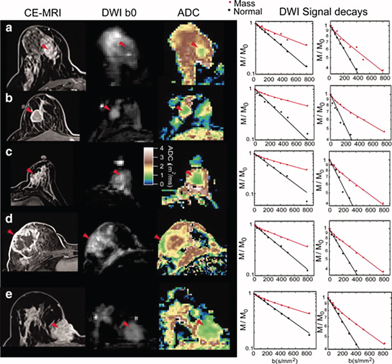
Tumor angiogenesis and cellular proliferation are important processes in breast cancer growth and metastasis. In terms of clinical application, the IVIM approach can separately reflect tissue diffusivity and tissue microcapillary perfusion in tissues without the need for contrast agents, with the advantage especially for patients contraindicated for contrast agents. Example IVIM signal decays from patients with breast lesions are shown in Fig. 8.5 .
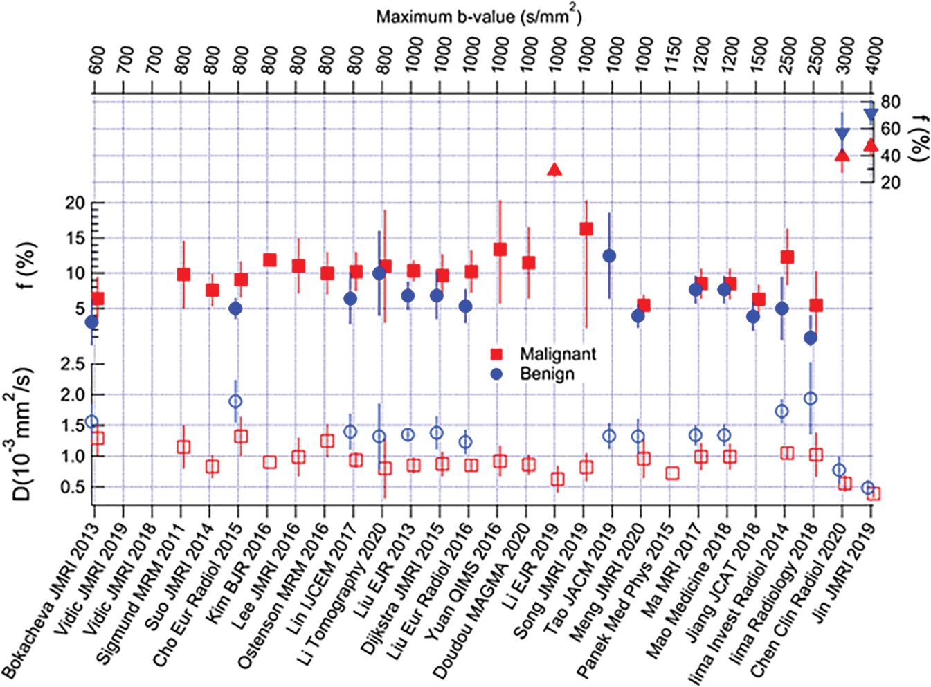
Many studies have reported the utility of IVIM for differentiating malignant from benign breast tumors, with higher f values in malignant compared with benign breast tumors. IVIM or combination of IVIM and non-Gaussian DWI parameters were reported to improve diagnostic accuracy over ADC alone, and the approach of combining parameters of IVIM, or IVIM and non-Gaussian (NG)–DWI to improve diagnostic accuracy, has been also explored.
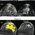
Many of these studies are illustrated in Fig. 8.6 , and a formal meta-analysis by Liang and colleagues summarized their collective implications as follows. In an analysis of 16 studies encompassing 1717 lesions, the diagnostic performance of IVIM and ADC parameters was considered in distinguishing benign from malignant lesions in terms of area under the curve (AUC), finding 0.85, 0.91, 0.85, and 0.81 for ADC, D, f , and D *, respectively. Thus the individual diagnostic performance of f or D met or exceeded that of ADC . Furthermore, the pooled analysis also showed IVIM parameters differentiated lesion histological subtype, grade, ER/PR/HER2/Ki-67 expression levels, and lymph node status, whereas ADC only differentiated histological subtype. This combined analysis, which incorporated studies with variable technical protocols, highlights the broad potential utility of IVIM. Detailed findings of individual studies are discussed further later.
IVIM Tumor Characterization: Subtypes, Molecular Prognostic Factors
Many IVIM studies have investigated the relationship between IVIM parameters and the hormone receptor status, HER2, and Ki-67 expression levels or molecular subtypes (luminal A, luminal B, HER2-positive, triple negative) of breast cancer. The IVIM parameters showing significant associations with the molecular prognostic factors or subtypes are shown in Table 8.1 .
| Investigator | Study Design | Year | Patients (n) | Field Strength | b values (s/mm 2 ) | ER | PR | HER2 | Ki-67 | Molecular Subtype |
|---|---|---|---|---|---|---|---|---|---|---|
| IVIM and non-Gaussian DWI models | ||||||||||
| Vidic´ et al. 28 | Prospective | 2018 | 51 | 3T | 0, 10, 20, 30, 40, 50, 70, 90, 120, 150, 200, 400, 700 | n/a | n/a | See subtype | n/a | Combined model distinguished ER+ HER2− from ER+ HER2+ with high accuracy (0.90) |
| Zhao et al. | Retrospective | 2018 | 119 | 3T | 0, 50, 100, 150, 200, 400, 500, 1000, 1500 | D *↓ | D *↓ | Fraction of D *↓ in luminal B (HER2−) D *; fraction of D *↑; D ↓ in triple negative | ||
| Suo et al. | Retrospective | 2017 | 101 | 3T | 0, 10, 30, 50, 100, 150, 200, 500, 800, 1000, 1500, 2000, 2500 | D , f , DDC, MD↓ | – | – | D *↑, α↓ | |
| Lee et al. | Retrospective | 2017 | 72 | 3T | 0, 25, 50, 75, 100, 150, 200, 300, 500,800 | D 50%, 75%, 90%, skewness↓, ADC 50%, mean, 75%, 90%, skewness↓- | ADC 75%↓ | D skewness↓ | f skewness↑ | Luminal < HER2-positive ( D 75th percentile, ADC 50%, ADC mean); luminal < triple negative < HER2-positive (ADC 75%, ADC 90%) |
| Difference in subtypes ( D skewness) | ||||||||||
| Kawashima et al. 32 | Retrospective | 2017 | 134 | 3 T | 0, 20, 40, 80, 120, 200, 400, 600, 800 | – | – | – | – | D and ADC lower; |
| Kim et al. | Prospective | 2016 | 275 | 3 T | 0, 30, 70,100, 150, 200, 300, 400, 500, 800 | D *↓ | D *↓, ADC↓, | – | D ↓ | Luminal A > other subtypes ( D ); Luminal A < other subtypes ( D *); luminal B (HER2−) < other subtypes (ADC); HER2-positive > other subtypes ( D *) |
| Cho et al. | Retrospective | 2016 | 50 | 3 T | 0, 30, 70, 100, 150, 200, 300, 400, 500, 800 | ADCmax↓, Dmax↓, DSD↓, D * kurtosis↓, D * skewness↓ | ADCmin↑, Dmin↑, DSD, D *max↓, D * skewness↓, f kurtosis↓, f skewness↓ | See subtypes | f skewness↓ | ER+ HER2− > other subtypes ( D * average); ER+ HER2− < other subtypes ( D * skewness, D * kurtosis); ER+ HER2+ < other subtypes (ADC kurtosis); ER+ HER2+ > other subtypes ( D skewness, D * kurtosis); triple negative > other subtypes ( D max) |
Related posts:
 DWI and Breast Physiology Status
 Disease and Treatment Monitoring
 Diffusion MRI as a Stand-Alone Unenhanced Approach for Breast Imaging and Screening
 Diffusion-Weighted Whole Body Imaging With Background Body Signal Suppression (DWIBS)
 Diffusion-Weighted Imaging (DWI) for Breast Lesion Characterization: The Olea Medical Perspective and the Utilization of Olea Sphere Software
 Breast Diffusion MRI Acquisition and Processing Techniques: The GE Healthcare Perspective
Stay updated, free articles. Join our Telegram channel

Full access? Get Clinical Tree


