Recent advances in magnetic resonance (MR) imaging have revolutionized peripheral nerve imaging and made high-resolution acquisitions a clinical reality. High-resolution dedicated MR neurography techniques can show pathologic changes within the peripheral nerves as well as elucidate the underlying disorder or cause. Neurogenic pain arising from the nerves of the pelvis and lumbosacral plexus poses a particular diagnostic challenge for the clinician and radiologist alike. This article reviews the advances in MR imaging that have allowed state-of-the-art high-resolution imaging to become a reality in clinical practice.
Key points
- •
The diagnosis of pelvic neuropathy is challenging for both radiologists and clinicians. Detailed knowledge of pelvic neural anatomy and of clinical syndromes and denervation patterns that commonly affect the pelvic nerves is crucial to the correct interpretation of magnetic resonance (MR) neurography studies. Advances in MR technology now enable high-resolution imaging of the lumbosacral plexus and its pelvic neural branches, with reliable visualization of many of the nerves commonly implicated in pelvic neuropathy.
- •
Appropriate use and interpretation of dedicated pelvic MR neurography may show pathologic changes within the peripheral nerves as well as elucidate the underlying disorder.
- •
In the case of negative MR neurography studies, other musculoskeletal disorders that may explain the patient’s clinical presentation may be shown. Recognition of potential pitfalls in MR neurography that may result in false-positive findings by the reporting radiologist is also crucial.
- •
The diagnostic performance of some of the MR findings that indicate neuropathy is yet to be established. Interpretation of MR neurography findings is best performed in conjunction with the clinical picture and in collaboration with the referring physician.
Introduction
Neurogenic pain arising from lumbosacral plexus and the nerves of the pelvis poses a particular diagnostic challenge for the clinician and radiologist alike, given the complexity of the anatomy, the frequent coexistent disorders and potential symptom generators, and the difficulty in obtaining high-resolution imaging while using a large field of view. Classic symptoms of pain corresponding with a particular nerve distribution are not always present and patients may have vague symptoms that can be attributed to a multitude of other disorders. The situation becomes even more confusing with involvement of multiple nerves, as seen in lumbar plexopathy. Lumbar discogenic pain and other disorders, such as hip osteoarthrosis, commonly coexist.
Until recently, imaging of peripheral nerves was limited from a technical standpoint, with no established gold standard imaging method to reliably visualize peripheral nerves and show disorders. With technical advances in magnetic resonance (MR) imaging, and particularly with the advent of dedicated high-resolution MR neurography, even small-caliber peripheral nerves and their associated disorders can now reliably be shown. Radiologists nevertheless may lack confidence and experience in reading dedicated high-resolution MR neurography examinations. By reviewing the basic principles and techniques of neural imaging, revisiting the relevant anatomy and highlighting common disorders, this article is intended to demystify this imaging technique along with its applications and interpretations, enabling the reader to apply it in daily clinical practice.
MR neurography: technical considerations
MR neurography is a tissue-specific imaging technique optimized for evaluating peripheral nerves, their internal fascicular morphology, alterations in neural signal and caliber, and associated space-occupying and other compressive lesions. Three-dimensional (3D) imaging is of critical importance in tracing the course of peripheral nerves, in identifying points of compression or disruption, and for preoperative planning. In general, MR neurography may either be T2 based or diffusion based. Diffusion-based MR imaging, especially diffusion tensor imaging, allows functional assessment of the nerves, but remains a novel technique, with specific hardware and software requirements to enhance the otherwise low signal/noise ratio (SNR) from these small nerves, limiting its application in routine clinical practice.
The Magnet
The strength of the magnet is an important consideration, with impact on both image quality and speed of acquisition. In general, there is superior performance of MR neurography at 3 T compared with 1.5 T, which has led us to only perform the technique using 3-T platforms. It is the advent of high-tesla imaging and its widespread availability that has facilitated the development of state-of-the-art MR neurography and made it a reality in daily clinical practice. Compared with 1.5-T MR imaging, 3-T MR imaging provides increased (nearly double) SNR, which in part is related to improved coil design, better gradient performance, and wider bandwidths. This improvement translates into higher spatial resolution and thinner slice sections with improved fluid conspicuity, as well as superior contrast/noise ratio, which improves anatomic characterization and lesion detection. Increased conspicuity of fluid and more uniform fat-suppression techniques result in better depiction of fascicular appearance of the nerves. There is also less inhomogeneity of the magnetic field. More robust hardware facilitates the application of multiple radiofrequency saturation pulses required for adequate vascular suppression. Furthermore, the application of parallel imaging allows faster acquisition times. It is difficult to produce quality T2-weighted 3D images on lower field strength magnets because of time and hardware limitations. 3D gradient echo sequences often have to be used, and images thus generated are frequently nonisotropic with poor SNR and soft tissue contrast and are prone to susceptibility artifacts. In contrast, high-quality isotropic 3D proton density and T2-weighted images can be acquired with relative ease and speed at 3 T and serve as an invaluable adjunct to two-dimensional (2D) images.
The Sequences
T1-weighted imaging
High-resolution T1-weighted imaging is excellent for depicting normal anatomy of the peripheral nerves and surrounding structures. Thin sections (maximum slice thickness of 4 mm), are necessary for adequate resolution of anatomic detail and fascicular morphology. Peripheral nerves appear as linear T1-hypointense structures, following an expected anatomic distribution. Differentiation from adjacent vessels is often possible, especially with the larger nerves, with arteries appearing as flow voids and veins appearing T1 hyperintense because of inflow phenomenon. With larger nerves or at higher resolution imaging, the individual fascicles may be resolved. Peripheral nerves are outlined by T1-hyperintense perineural fat, with a characteristic reverse tram track appearance of alternating T1-hyperintense and T1-hypointense signal, which increases their conspicuity. Infiltration of the perineural fat and soft tissues is often best depicted on T1-weighted imaging. The presence of muscle fatty replacement in the setting of long-standing denervation is also seen to best advantage on this imaging sequence.
T2-weighted imaging
Pathologic changes within the nerve are seen to best advantage on T2-weighted imaging. In addition, many mass lesions and pathologic processes that commonly result in neural compression (eg, paralabral and ganglion cysts, peripheral nerve sheath tumors, fluid-filled bursae) are best characterized and are most conspicuous on T2-weighted imaging. With standard fast spin echo (non–fat suppressed) T2-weighted imaging, it is difficult to discern abnormal increased T2 signal from perineural and intraneural fat, therefore fat-suppressed T2-weighted imaging is the optimal sequence for detecting neural disorders. This imaging sequence is also most sensitive for early changes of muscle denervation signal alterations. However, there are drawbacks to fat-suppressed T2-weighted imaging with more artifact from hyperintense vascular structures and partial volume averaging. Vascular structures, which typically accompany the nerve, appear hyperintense and may be confused with neural signal abnormality or perineural edema.
Dedicated MR neurography uses increased T2 weighting with thinner slices, to both increase conspicuity of T2 signal change and achieve higher spatial resolution. Maximizing the conspicuity of increased T2 signal in nerves is achieved in 3 ways: (1) using sequences with long echo times (TEs) (90–130 ms), (2) applying radiofrequency saturation pulses to suppress signal from adjacent vessels, and (3) using frequency-selective or adiabatic inversion recovery imaging–type fat suppression. This result is best achieved at higher field strength, emphasizing the importance of technological advances in the development of high-resolution neural imaging. This technique results in increased T2 weighting, minimizes spurious signal from adjacent vessels and fat, and is more sensitive for showing neural signal abnormality. Newer techniques used in 3D imaging, namely steady-state free precession and diffusion techniques, result in superior suppression of vascular signal in T2-weighted sequences, particularly when imaging the extremities.
3D Imaging
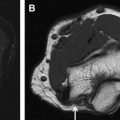
Isotropic 3D imaging is an essential component of state-of-the-art MR neurography. Nerves often follow oblique courses and are not seen to best advantage on standard axial, coronal, and sagittal imaging planes. 3D multiplanar reconstructed (MPR), curved planar reconstructed (CPR), and maximal intensity projected (MIP) images greatly facilitate the visualization of nerves and are particularly useful for preoperative planning. Decreased magic angle artifact and partial volume averaging on 3D imaging allow more accurate depiction of disorders. Furthermore, caliber and signal change in nerves, which may be subtle or attributed to volume averaging on axial imaging, are seen to better advantage in the longitudinal plane, allowing better assessment of the extent of the abnormality. Certain disorders, such as plexiform neurofibromata, particularly lend themselves to 3D imaging for depiction of the disease burden in one image ( Fig. 1 ). Compression of peripheral nerves by disc protrusions, space-occupying lesions, and anatomic fibro-osseous tunnels is also more accurately delineated on 3D imaging. Focal interruption of a nerve can be particularly challenging to show on axial imaging, and 3D reconstructions may prove crucial in this scenario. Variations in muscular volume and anatomy may also be better assessed on 3D imaging.
Several techniques may be used in 3D imaging. SPACE (sampling perfection with application optimized contrasts by using different flip angle evolutions, Siemens, Erlangen, Germany) sequence is an isotropic single-slab acquisition, mainly spin echo–type sequence that allows MPR, CPR, and MIP reconstructed images to map out the peripheral nerves and associated disorder in the longitudinal plane. This imaging may be obtained in spectral adiabatic inversion recovery (SPAIR) or short tau inversion recovery sequence (STIR) contrasts, thus providing T2 weighting and optimizing sensitivity for detecting neural disorders. STIR imaging is preferred for imaging of the lumbosacral and brachial plexus because of superior fat suppression, whereas SPAIR imaging is preferred for imaging of the extremities. More recent developments include the 3D diffusion-weighted (DW) reversed fast imaging with steady-state free precession (PSIF) sequence, which is a heavily T2-weighted technique, combining selective suppression of vascular flow signal with multiplanar capabilities. The PSIF sequence holds great promise, particularly in the imaging of the extremities. Attempts to suppress vascular flow signal with the application of saturation bands usually fails in peripheral locations, either because of the slow or in-plane flow within the peripheral vessels, or because of the variable oblique courses of peripheral neurovascular bundles. PSIF, because of its sensitivity to flow-related dephasing of the transverse magnetization, causes vessels in the imaging field of view to lose their signal intensity. Vascular signal suppression is also enhanced by the small diffusion moment applied to this sequence ( Fig. 2 ).
The Field of View
Large field of view is most commonly used in pelvic neurography protocols, and it occurs at the expense of resolution but allows side-to-side comparison and evaluation of multiple nerve distributions on a single study. In our experience, the nerves most commonly affected in pelvic neuropathy can be reliably shown when a dedicated MR neurography protocol is performed. In large patients, and when a particularly large field of view is required, 3D STIR-SPACE imaging may be preferable to 3D SPAIR-SPACE imaging given the superior and more robust fat suppression.
Pitfalls and Technical Limitations
Magic angle effect, a well-described phenomenon in imaging of tendons, also occurs when imaging peripheral nerves. This effect results in spurious increased signal when the nerve lies in a plane 55° to the main vector of the magnet. Unlike tendons, this effect may persist in nerves, even at longer TEs (>66 milliseconds) and therefore higher TEs must be used to overcome it. The interpreting radiologist was traditionally advised to be particularly aware of this phenomenon when reporting increased intraneural T2 signal in MR neurography studies; however, recent literature concludes that magic angle effect is a rare source of false-positive interpretation on MR neurography, particularly in nerves that run parallel to the main vector of the magnet.
Despite the use of suppressive radiofrequency pulses, hyperintense vascular signal is often present on MR neurography examinations, especially at high TE, which is a particular source of confusion in small nerves when it occurs in the accompanying vascular bundle and may be misinterpreted as neural or perineural signal abnormality. Inhomogeneous fat suppression is another potential source of error, particularly in the pelvis, given the large field of view and the high number of patients who have hip or lumbar instrumentation, which further degrades the local magnetic field thus worsening fat suppression. Increased susceptibility and chemical shift artifact, also seen at 3 T, may be counteracted by shortening the ET, performing parallel imaging, and increasing the bandwidth. Nonetheless, 1.5-T imaging may be preferable when evaluating nerves in close proximity to a metal prosthesis. Specific absorption rate limits are reached earlier at 3 T compared with 1.5 T because there is increased energy deposition for radiofrequency excitation at 3 T. However, this difference is usually balanced by faster image acquisition and shorter examination time and does not usually pose a clinical problem. Other potential drawbacks of 3D imaging include longer imaging times, and time spent producing and interpreting multiplanar reformatted images ( Box 1 ).
Differentiating nerves from adjacent vessels
Increased perineural T2 signal from adjacent vessels
Magic angle effect
Inhomogeneous fat suppression
Increased specific absorption rate (SAR) at 3 T
Increased susceptibility artifact at 3 T
Anatomic considerations
Lumbosacral Plexus
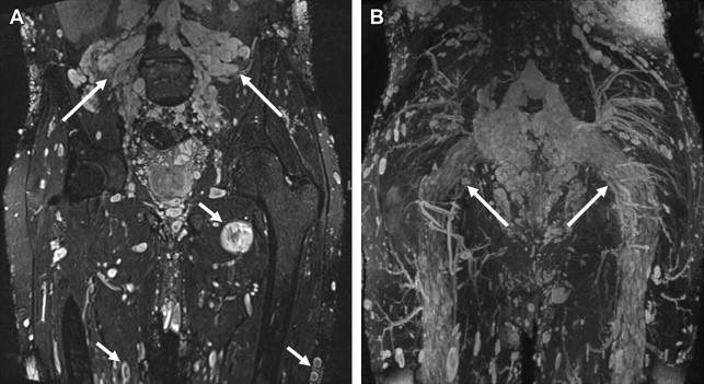
The lumbosacral plexus is composed of a lumbar and sacral plexus ( Fig. 3 ). The lumbar plexus is formed from the ventral rami of L1 to L4 and a small contribution from the 12th thoracic nerve. The plexus descends dorsally or within the psoas muscle. Branches emerging from the lateral border of the psoas muscle include the iliohypogastric, ilioinguinal, genitofemoral, lateral femoral cutaneous, and femoral nerves, whereas branches emerging from the medial border of the psoas muscle include the obturator nerve and lumbosacral trunk. A minor branch of L4 combines with the ventral ramus of L5 to form the lumbosacral cord or trunk. The latter descends over the sacral ala and joins the S1 to S3 nerve roots on the anterior aspect of the piriformis muscle to form the sacral plexus. Thus the sacral plexus is formed from L4 to S4 ventral rami. The sciatic, inferior, and superior gluteal and pudendal nerves constitute its sacral branches. Lumbosacral plexus muscular innervations by nerve root are listed in Table 1 and the most clinically important motor and sensory innervations of multiple peripheral nerves of the lower limb and pelvis are discussed in more detail later.
| T12 | L1 | L2 | L3 | L4 | L5 | S1 | S2 | S3 | S4 | S5 | |
|---|---|---|---|---|---|---|---|---|---|---|---|
| Obturator internus | * | * | |||||||||
| Obturator externus | * | * | * | ||||||||
| Pectineus | * | * | * | ||||||||
| Psoas major | * | * | * | * | * | ||||||
| Iliacus | * | * | * | * | * | ||||||
| Iliopsoas | * | * | * | ||||||||
| Gluteus minimus | * | * | |||||||||
| Gluteus medius | * | * | |||||||||
| Gluteus maximus | * | * | |||||||||
| Piriformis | * | * | |||||||||
| Adductor brevis | * | * | * | ||||||||
| Adductor longus | * | * | |||||||||
| Adductor magnus | * | * | |||||||||
| Levator ani | * | * | * |
Sciatic Nerve
The sciatic nerve is the largest peripheral nerve in the body and is reliably shown on computed tomography (CT) and MR imaging. It is formed from the L4 to S3 nerve roots and may descend anterior to (most commonly), above, or within the piriformis muscle. After exiting the pelvis through the greater sciatic foramen, it descends in the thigh between the adductor magnus and the gluteus maximus muscles ( Fig. 4 ). The sciatic nerve is composed of the medial tibial and the lateral common peroneal divisions, which provide motor innervation to the posterior thigh muscles and all motor function below the knee (anterior, lateral, posterior, and deep muscular compartments). It gives all sensory innervation to the lower limb with the exception of medial sensory innervation of the thigh and leg, which is provided by the obturator and femoral nerves.
Superior and Inferior Gluteal Nerves
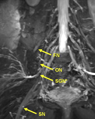
The superior gluteal nerve is formed from the posterior roots of L4, L5, and S1. It exits the pelvis, curving under the roof of the greater sciatic foramen above the piriformis muscle, and then passes between the gluteus minimus and gluteus medius muscles before giving off superior and inferior branches ( Fig. 5 ). The superior branch terminates in the gluteus minimus muscle and the inferior branch terminates in the tensor fascia lata. The superior gluteal nerve acts to abduct the thigh at the hip by providing motor innervation to the gluteus minimus, gluteus medius, and tensor fascia lata muscles.
The inferior gluteal nerve formed from the posterior roots of L5, S1, and S2 provides motor innervations to the gluteus maximus, which, with the aid of the hamstrings, acts to extend the thigh. It exits the pelvis through the sciatic notch passing below the piriformis muscle and lies medial to the sciatic nerve before its terminal branch provides motor innervation to the gluteus maximus muscle. The superior and inferior gluteal nerves have no sensory contribution.
Lateral Femoral Cutaneous Nerve
The lateral femoral cutaneous nerve arises from L2 and L3, descends lateral to the psoas muscle, crosses the iliacus muscle deep to its fascia, and passes either through or underneath the lateral aspect of the inguinal ligament to the lateral thigh where it divides into anterior and posterior branches ( Fig. 6 ). It innervates the skin on the lateral aspect of the thigh and, as its name implies, is purely sensory.