MRI Perfusion-Weighted Imaging Analysis

Dynamic susceptibility contrast MRI (DSC-MRI) is one of the most commonly used functional MRI methods for studying cerebral perfusion parameter change. This method has many clinical applications, including diagnosis of brain neoplasms and cerebrovascular disease, studying of the vasodilatory capacity of brain during cerebral perturbation, and assessment of the risk of infarct progression in acute stroke. Since it first appeared in middle of the 1980s, it has been widely employing to quantify blood flow parameters such as cerebral blood flow (CBF), cerebral blood volume (CBV), mean transit time (MTT), and tissue permeability. However, to estimate these parameters accurately, we need to smooth the concentration time course by fitting it with a distribution function such as gamma-variate function. Furthermore, if we want to measure these cerebral parameters absolutely, we need to segment arterial input function (AIF). This is because cerebral tissue concentration time course is the convolution between AIF and the residual function. Therefore, to compute the residual function, we must solve the well-known ill-posed inverse problem for deconvolution calculation. The purposes of this chapter are to address all these issues from a numerical analysis viewpoint. In particular, we firstly review the indicator–dilution theory which DSC-MRI is depended on. Second, linear and nonlinear regression methods for gamma-variate fits are presented and compared for the CBF parameter calculation. Third, a new robust method is proposed to determine AIF from the whole brain for absolute quantification. Finally, to solve the ill-posed problem in perfusion-weighted imaging (PWI) analysis, we develop an adaptive method, i.e., linear piecewise method to estimate the ridge regression parameter for PWI regularization. After residual function is determined, CBF, CBV, and MTT can be computed according to indicator–dilution theory.

Keywords

Perfusion-weighted imaging (PWI)Cerebral blood flow (CBF) parametersNonlinear regression analysisArterial input function (AIF)Gamma-variate fittingDeconvolutionIll-posed inverse problem

1.1 Perfusion Imaging

Cerebrovascular diseases are among the leading causes of illness and death in the industrial nations [1]. These diseases are related to the blood vessels supplying the brain; thus, we can study blood flow parameters to diagnose and assess these diseases and its progression. However, in terms of both medical equipment and image analysis methods, quantification of these parameters that characterize cerebral microcirculation is difficult. Although numerous techniques such as positron emission tomography (PET) have been devised to measure cerebral blood flow (CBF) parameters, dynamic susceptibility contrast MRI (DSC-MRI) offers several advantages, i.e., no ionizing radiation, high spatial resolution, and low relative cost. For this reason, we will introduce the numerical analysis methods for processing DSC-MRI data, although these ideas can also been applied to PET data and computed tomography (CT) data analysis.

In MRI perfusion-weighted imaging (PWI) study, the major goals are to determine CBF, cerebral blood flow (CBV), mean transmit time (MTT), and tracer arrival time. Because tracer delay or arrival time is an important parameter for cerebral vascular disease studies, it is necessary to estimate it from concentration time course using the linear or nonlinear regression analysis methods objectively. We regard tracer delay as an optimal parameter in the gamma-variate function, which can be estimated using a nonlinear iterative numerical method. We give mathematical details to achieve nonlinear regression for gamma-variate fitting in this chapter.

There are two methods to quantify CBF, CBV, and MTT, i.e., relative quantification and absolute quantification methods [2, 3]. For the former, it does not need to estimate the arterial input function (AIF) for these parameters estimation, but it has the limitation of difficult to compare between subjects and follow-up studies on the same subject. To circumvent these limitations, great effects have been devoted to quantify these parameters absolutely for easier intra- and intersubject comparisons. However, to quantify of the CBF, CBV, and MTT absolutely, one needs to select AIF [4] either manually or by means of automatic segmentation algorithms. Manual selection has limitations, i.e., it needs a trained operator, time consuming, and subjective judgment. The automatic method has the advantages of faster and objective, but it is sensitive to noise. In this chapter, we introduce a new algorithm to achieve reliable and robust AIF segmentation.

After AIF has been chosen, residual function can be estimated from the deconvolution between tissue concentration time course and AIF. Because the deconvolution calculation in PWI is an ill-posed problem, regularization is needed to adjust the estimation to give meaningful results. Although ridge regression and general cross-validation (GCV) methods have been proposed to solve this problem [5, 6], these methods, however, are computationally demanding and difficult to apply on a voxel by voxel base. To overcome this limitation, we suggest a piecewise linear method to achieve faster and adaptive regularization for PWI calculation. After residual function has been estimated, CBF, CBV, and MTT can be easily calculated based on the fitted concentration–time curves [1, 3].

Because absolute quantification of these CBF parameters from DSR-MRI study is based on indicator–dilution theory, we start with introducing the theory, and then we detail each step to calculate cerebral vascular parameters.

1.1.1 Indicator–Dilution Theory for DSC-MRI

The indicator–dilution theory has long been used in metabolic and circulatory studies, and most techniques to investigate CBF are relied on it, and DSC-MRI is no exception. To introduce the theory, let m units of indicator be injected, C(t) the concentration of indicator, and dm the amount of indicator leaving the system during a small time interval between t and t + dt. In a short period of time dt, the amount of tracer quantity brought into the system would be equal to the amount carried away; based on this, we have [7–10]

$\mathrm{d}m= FC(t)\mathrm{d}t$

(1.1)

where F is blood flow in units of volume/time. Calculating integration from both sides of the above equation, we get

${\int}_0^{\infty }1}\mathrm{d}m=m={\displaystyle {\int}_0^{\infty } FC(t)\mathrm{d}t}=F{\displaystyle {\int}_0^{\infty }C(t)\mathrm{d}t$

(1.2)

We introduce probability density function of the transit times, h(t), which describes the fraction of injected indicator leaving the system per unit time at time t, i.e.,

$h(t)=\frac{ FC(t)}{m}$

(1.3)

As h(t) is probability density function and all the fluid entering the system at 0 time must eventually leave, we have [10]

${\displaystyle {\int}_0^{\infty }h(t)\mathrm{d}t}=1$

(1.4)

This property can be obtained from Eqs. (1.2) and (1.3). We define the MTT as the first moment of h(t), i.e.,

$\mathrm{MTT}=E\left(h(t)\right)={\displaystyle {\int}_0^{\infty } th(t)\mathrm{d}t}$

(1.5)

where E is expectation operation. Furthermore, we define the residual function r(t) as

$r(t)=\left\{\begin{array}{ll}1-{\displaystyle {\int}_0^th(t)\mathrm{d}t},\hfill & t\ge 0\hfill \\ {}1,\hfill & t<0\hfill \end{array}\right.$

(1.6)

It is easy to see that r(0) = 1 and r(∞) = 0, suggesting that the residual function decreases continuously and smoothly from 1 to 0. This function quantifies the relative amount of contrast agent that is still inside the volume of interest (VOI) at the t after an idealized delta-shaped contrast agent bolus has entered the volume at the arterial inlet at time t = 0, i.e., C _art(t) = δ(t).

From Eq. (1.2) and let m _in(t) and m _out(t) denote the accumulated masses of contrast agent that have entered and left the volume of interest during the time interval [0,t], respectively, we have [11]

$\left\{\begin{array}{l} {m}_{\mathrm{in}}(t)=F{\displaystyle {\int}_0^{\infty }{C}_{\mathrm{art}}}\left(\tau \right)\mathrm{d}\tau \\[9pt] {m}_{\mathrm{out}}(t)=F{\displaystyle {\int}_0^{\infty }{C}_{\mathrm{ven}}}\left(\tau \right)\mathrm{d}\tau \hfill \end{array}\right.$

(1.7)

The volume flow F is assumed to be constant over time. C _art(t) and C _ven(t) are the contrast agent concentrations at the arterial inlet and the venous outlet, respectively. Based on the principle of conservation of mass, we can compute the mass of a contrast agent within VOI at time t as

$m(t)={m}_{\mathrm{in}}(t)-{m}_{\mathrm{out}}(t)=F{\displaystyle {\int}_0^t\left({C}_{\mathrm{art}}\left(\tau \right)-{C}_{\mathrm{ven}}\left(\tau \right)\right)\mathrm{d}\tau }.$

(1.8)

Because the contrast agent concentration C _ven(t) at the venous outlet can be calculated from the contrast agent concentration C _art(t) at the arterial inlet by convolving it with h(t), we get

${C}_{\mathrm{ven}}(t)={\displaystyle {\int}_{-\infty}^{+\infty }{C}_{\mathrm{art}}\left(\tau \right)}h\left(t-\tau \right)\mathrm{d}\tau$

(1.9)

and

${C}_{\mathrm{art}}(t)={\displaystyle {\int}_{-\infty}^{+\infty }{C}_{\mathrm{art}}\left(\tau \right)}\delta \left(t-\tau \right)\mathrm{d}\tau$

(1.10)

Substitute Eqs. (1.9) and (1.10) into Eq. (1.8), we get

$m(t)=F{\displaystyle {\int}_0^t\left({\displaystyle {\int}_{-\infty}^{+\infty }{C}_{\mathrm{art}}\left(\xi \right)\delta \left(\tau -\xi \right)\mathrm{d}\xi }-{\displaystyle {\int}_{-\infty}^{+\infty }{C}_{\mathrm{art}}\left(\zeta \right)h\left(\tau -\xi \right)}\mathrm{d}\xi \right)\mathrm{d}\tau }$

(1.11)

Swap the order of integration and rearranging the equation leads to

$m(t)=F{\displaystyle {\int}_{-\infty}^{+\infty }{C}_{\mathrm{art}}\left(\xi \right)\left({\displaystyle {\int}_0^t\left(\delta \left(\tau -\xi \right)-h\left(\tau -\xi \right)\right)\mathrm{d}\tau}\right)\mathrm{d}\xi }$

(1.12)

Substitute τ′ = τ − ξ and use

$r(t)=1-{\displaystyle {\int}_0^th\left(\tau \right)\mathrm{d}\tau }={\displaystyle {\int}_0^t\left(\delta \left(\tau \right)-h\left(\tau \right)\right)\mathrm{d}\tau }$

(1.13)

Using h(t) = 0 for t < 0, we get

${\int}_0^t\left(\delta \left(\tau -\xi \right)-h\left(\tau -\xi \right)\right)\mathrm{d}\tau }={\displaystyle {\int}_{-\xi}^{t-\xi}\left(\delta \left({\tau}^{\prime}\right)-h\left({\tau}^{\prime}\right)\right)\mathrm{d}{\tau}^{\prime }=r\left(t-\xi \right)$

(1.14)

Substituting Eq. (1.14) into (1.12), we obtain

$m(t)=F{\displaystyle {\int}_{-\infty}^{+\infty }{C}_{\mathrm{art}}\left(\xi \right)r\left(t-\xi \right)\mathrm{d}\xi }$

(1.15)

We define the CBF as the net blood flow through the voxel/VOI divided by the mass of the voxel/VOI:

$\mathrm{CBF}=\frac{F}{ V\rho}$

(1.16)

where ρ is density and V is the volume of blood for the consideration. Inserting Eq. (1.16) into (1.15) yields

$\frac{m(t)}{V}=\mathrm{CBF}\cdot \rho \cdot {\displaystyle {\int}_{-\infty}^{+\infty }{C}_{\mathrm{art}}\left(\xi \right)r\left(t-\xi \right)\mathrm{d}\xi }$

(1.17)

Because we define the contrast agent concentration C(t) within the VOI as

$C(t)=\frac{m(t)}{V}$

(1.18)

which leads to the following formulation of the indicator–dilution theory:

$C(t)=\frac{m(t)}{V}=\mathrm{CBF}\cdot \rho \cdot {\displaystyle {\int}_{-\infty}^{+\infty }{C}_{\mathrm{art}}\left(\xi \right)r\left(t-\xi \right)\mathrm{d}\xi }=\rho \cdot \mathrm{CBF}\cdot \left({C}_{\mathrm{art}}(t)\otimes r(t)\right)$

(1.19)

where ⊗ represents the convolution operation.

1.1.2 MTT and CBV Calculation

In order to calculate MTT, we introduce an intermediate variable, the flow-scaled residue function:

$R(t)=\rho \cdot \mathrm{CBF}\cdot r(t)$

(1.20)

which is given in units of 1/s and can be determined directly from the measured data C _art(t) and C(t) through deconvolution operation. From Eqs. (1.19) and (1.20), we get

$C(t)={C}_{\mathrm{art}}(t)\otimes R(t)$

(1.21)

Using the property of the residual function, i.e., r(0) = 1 = max(r(t)), from Eq. (1.20), we get CBF as

$\mathrm{CBF}=\frac{ \max \left(R(t)\right)}{\rho }$

(1.22)

Another perfusion parameter, the time-to-maximum (T-max) of the flow-scaled residual function can be determined as

$\mathrm{T}\kern0.5em \max =\underset{t}{ \arg \kern0.5em \max \left(R(t)\right)}$

(1.23)

Furthermore, we calculate the derivative to t from both sides of Eq. (1.6), and we have

$\frac{\mathrm{d}r(t)}{\mathrm{d}t}=-h(t)$

(1.24)

Substituting Eq. (1.24) into (1.5), we get

$\begin{aligned}[b]\mathrm{MTT}&={\displaystyle {\int}_0^{\infty }t\left(-\frac{\mathrm{d}r(t)}{\mathrm{d}t}\right)}\mathrm{d}t\\ &=-{\displaystyle {\int}_0^{\infty }t}\mathrm{d}r(t)\\ &={\left.-r(t)t\right|}_0^{\infty }+{\displaystyle {\int}_0^{\infty }r(t)\mathrm{d}t}\\ &={\displaystyle {\int}_0^{\infty }r(t)\mathrm{d}t}\end{aligned}$

(1.25)

On the other hand, calculating integration from both sides of Eq. (1.20), we obtain

${\int}_0^{\infty }r(t)\mathrm{d}t}=\frac{{\displaystyle {\int}_0^{\infty }R(t)}}{\rho \cdot \mathrm{CBF}$

(1.26)

Inserting Eq. (1.22) into (1.26), we finally get MTT from Eq. (1.25) as

$\mathrm{MTT}=\frac{{\displaystyle {\int}_0^{\infty }R(t)}}{ \max \left(R(t)\right)}$

(1.27)

Since we have gotten CBF and MTT from Eqs. (1.22) and (1.27), respectively, we can calculate CBV using central volume theorem as

$\mathrm{CBV}=\mathrm{MTT}\cdot \mathrm{CBF}=\frac{{\displaystyle {\int}_0^{\infty }R(t)\mathrm{d}t}}{\rho }$

(1.28)

An alternative method to compute CBV is based on the assumption that the average contrast agent concentration C(t) in the tissue volume can be related to the average contrast agent concentration C _cap(t) in the capillary bed by

$C(t)=\left(\rho \cdot \mathrm{CBV}\right)\cdot {C}_{\mathrm{cap}}(t)$

(1.29)

According to the principle of conservation of mass, it follows that

$m=F{\displaystyle {\int}_0^{\infty }{C}_{\mathrm{art}}(t)\mathrm{d}t}=F{\displaystyle {\int}_0^{\infty }{C}_{\mathrm{cap}}(t)\mathrm{d}t}=F{\displaystyle {\int}_0^{\infty }{C}_{\mathrm{ven}}(t)\mathrm{d}t}$

(1.30)

where m is the total mass of contrast agent that has passed through the ROI. Calculating the integration from both sides of Eq. (1.29) between [0,∞] interval, substituting Eq. (1.30) into (1.29), and rearranging the equation, we have [12]

$\mathrm{CBV}=\frac{1}{\rho}\frac{{\displaystyle {\int}_0^{\infty }C(t)\mathrm{d}t}}{{\displaystyle {\int}_0^{\infty }{C}_{\mathrm{art}}(t)\mathrm{d}t}}=\frac{1}{\rho}\frac{{\displaystyle {\int}_0^{\infty }C(t)\mathrm{d}t}}{{\displaystyle {\int}_0^{\infty }{C}_{\mathrm{ven}}(t)\mathrm{d}t}}$

(1.31)

Finally, a maximum slop method which is a nondeconvolution based has been proposed for CBV calculation [13]. The idea of this method is to approximate integration in Eq. (1.31) using its maximum values, i.e.,

$\mathrm{CBV}=\frac{ \max \left(C(t)\right)}{ \max \left({C}_{\mathrm{ven}}(t)\right)}$

(1.32)

For the sake of simplicity, this method assumes that there is no venous outflow from the tissue volume under consideration during the time of observation. From Eq. (1.8), set C _ven(t) = 0, and we obtain

$m(t)=F{\displaystyle {\int}_0^{\infty }{C}_{\mathrm{art}}(t)\mathrm{d}t}$

(1.33)

Considering Eqs. (1.15, 1.16, 1.17, and 1.18), we have

$C(t)=\rho \cdot \mathrm{CBF}\cdot {\displaystyle {\int}_0^t{C}_{\mathrm{art}}\left(\tau \right)\mathrm{d}\tau }$

(1.34)

Taking the derivative of (1.34) yields

${\left[\frac{\mathrm{d}C(t)}{\mathrm{d}t}\right]}_{\max }=\rho \cdot \mathrm{CBF}\cdot {\left[{C}_{\mathrm{art}}(t)\right]}_{\max }$

(1.35)

which suggests that CBF can be estimated by dividing the maximum slope of the tissue concentration time. An advantage of this method is the shorter overall acquisition time; as a downside, it requires a faster contrast agent bolus injection rate to approximately fulfill the no-venous-outflow condition anisotropy than gray matter.

1.1.3 DSC-MRI Time Series Analysis

The indicator–dilution theory in previous sections is borrowed from CT and PET studies; to use this theory for MRI perfusion study, we need to convert the measured DSC-MRI signal to tracer concentration. Studies have been shown that the DSC-MRI signal intensity can be converted to gadolinium diethylene triamine pentaacetic acid (Gd-DTPA) concentration using [14]

$C(t)=-k\cdot \ln \frac{S(t)}{S_0}$

(1.36)

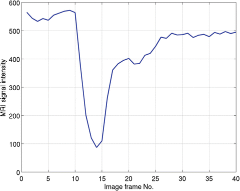
whereC(t) is the measured concentration of Gd-DTPA with respect to time and k is a constant that is inversely proportional to echo time (TE), depending on the MR scanner (for simplicity, a value of 1 for k is assumed throughout the study). S(t) is the MRI signal intensity with respect to time, and S ₀ is the baseline MRI signal before the presence of Gd-DTPA and after steady-state magnetization has been achieved (Fig. 1.1). In this study, we estimated S ₀ by averaging first several images before the tracer appearance from the brain perfusion image sequence. Using robust statistic trim mean method [15], it can be calculated as

Fig. 1.1

MRI signal intensity changes with time

${S}_0=\mathrm{Tr}\kern0.5em \mathrm{Mean}\left({S}_{01},{S}_{02},\dots, {S}_{0N},r,s\right)=\frac{1}{N-1-r-s}{\displaystyle \sum_{i=r+1}^{N-s}{S}_0(i)}$

(1.37)

where S ₀₁, S ₀₂, …, S _0Nis the N time points in the concentration–time curve and r and s are the number of largest and smallest values in the N − 1 time points. We set N = 8 and rejected the largest and smallest value in the N − 1 time points, so we set r = s = 1.

Figure 1.1 shows one typical MRI signal changes with time at one randomly selected voxel in one of our human brain data (see Appendix C), where x-axis is the MRI image frames and y-axis is the MRI signal intensity. In this example, S ₀ represents the MRI images from 1 to 8, and S(t) denotes the rest of MRI images. It is clear that the magnitude of the signal decrease rapidly between the 10th and 14th MRI image frame. This decrease of signal intensity is caused by the appearing of the Gd-DTPA (tracer). Then, due to the tracer density reduction, the signal increases from MRI image from No. 14 to No. 20. We call this process as the first passage of contrast agent. After that, the second passage of contrast agent begins from the No. 20th image approximately, but it is difficult to estimate the ending time of the second passage in this case, although there are some studies using this information for CBF parameter calculation.

After DSC-MRI image time series have been collected, applying robust statistics as given in Eq. (1.37), we obtained estimated S ₀ for concentration time course calculation. Substituting S ₀ into Eq. (1.36), we get the concentration time course. Figure 1.1 shows MRI signal intensity, and using Eq. (1.36), we can convert the signal into Gd-DTPA concentration as displayed in Fig. 1.2 (dotted curve). Because we calculate negative logarithm of the signal as shown in Eq. (1.36), the signal changes directions, i.e., the minimum value in Fig. 1.1 becomes the maximum value in Fig. 1.2. Furthermore, this curve looks roughly like a gamma distribution from visual inspection. Indeed, it has been reported that the concentration time course from DSC-MRI can be smoothed by applying gamma-variate fitting [16].

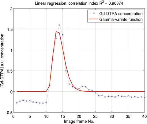
Fig. 1.2

An example of concentration time course (Obtained from Fig. 1.1) and its linear gamma-variate fit result. K = 0.5186, α = 4.5809, β = 0.7480, t ₀ = 9.5, t _e = 16, t _m = 14, and FWHM = 4

1.2 Gamma-Variate Fitting

A number of theoretical and empirical mathematical expressions for concentration time course C(t) have been suggested. For instance, lognormal function [17], local density random walk (LDRW) model [18], and gamma-variate model [16] have been applied for perfusion studies. However, from experimental observation, gamma-variate function bears a remarkable resemblance to indicator–dilution curves from DSC-MRI (see Fig. 1.2). Due to its simplicity, gamma-variate is becoming the most commonly used functions for indicator–dilution studies in DSC-MRI time series analysis. This is because the temporal resolution in PWI is generally low, and only a few time points are available to estimate the model parameters. Thus, gamma function model, which is simpler, provides greater advantages than other functions to smooth concentration time course.

There are two basic roles to fit the concentration time course: one is to exclude the tracer recirculation effects and the other is to smooth the concentration time course for quantification cerebrovascular parameters [19–21]. The gamma-variate function can be expressed as [16, 22]

$$$ C(t)=K{\left(t-{t}_0\right)}^{\alpha } \exp \left(-\frac{t-{t}_0}{\beta}\right),\kern1em t>{t}_0 $$ ” src=”/wp-content/uploads/2016/04/A317179_1_En_1_Chapter_Equ38.gif”></DIV></DIV><br /> <DIV class=EquationNumber>(1.38)</DIV></DIV>else <SPAN class=EmphasisTypeItalic>C</SPAN>(<SPAN class=EmphasisTypeItalic>t</SPAN>) = 0</DIV><br /> <DIV class=Para>where <SPAN class=EmphasisTypeItalic>K</SPAN> is constant scale factor; <SPAN class=EmphasisTypeItalic>α</SPAN>, <SPAN class=EmphasisTypeItalic>β</SPAN> are gamma-variate parameters; <SPAN class=EmphasisTypeItalic>t</SPAN> <SUB>0</SUB> is the tracer arrival time; and <SPAN class=EmphasisTypeItalic>K</SPAN>, <SPAN class=EmphasisTypeItalic>α</SPAN>, <SPAN class=EmphasisTypeItalic>β</SPAN>, and <SPAN class=EmphasisTypeItalic>t</SPAN> <SUB>0</SUB> are optimal parameters to be estimated.</DIV><br /> <DIV id=Sec6 class=$

1.2.1 Linear Regression Method for Gamma-Variate Fitting

Two methods, i.e., linear and nonlinear regression methods, can be employed to estimate the parameters in Eq. (1.38) for PWI study. We begin with linear method for the gamma-variate parameters estimation, and then we will give details of the nonlinear method for the fitting. Based on the assumption that the model error is homoscedasticity, we can linearize the gamma-variate function (Eq. (1.38)) by taking logarithms from both sides of Eq. (1.38), yielding [23]

$$$ \ln \left(C(t)\right)= \ln (K)+\alpha \kern0.5em \ln \left(t-{t}_0\right)-\frac{1}{\beta}\left(t-{t}_0\right),\kern1em t>{t}_0 $$ ” src=”/wp-content/uploads/2016/04/A317179_1_En_1_Chapter_Equa.gif”></DIV></DIV></DIV>or<br /> <DIV id=Equ39 class=Equation><br /> <DIV class=EquationContent><br /> <DIV class=MediaObject><IMG alt=$

(1.39)

where y _i = ln(C(t _i)), b ₀ = ln(K), b ₁ = α, ${b}_2=-\frac{1}{\beta }$ , x _i1 = ln(t _i − t ₀), and x _i2 = t _i − t ₀. Then Eq. (1.39) can be expressed as

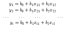$\begin{array}{c}{y}_1={b}_0+{b}_1{x}_{11}+{b}_2{x}_{12}\\ {}{y}_2={b}_0+{b}_1{x}_{21}+{b}_2{x}_{22}\\ {}\dots \kern2em \dots \kern2em \dots \kern3.5em \dots \\ {}{y}_i={b}_0+{b}_1{x}_{i1}+{b}_2{x}_{i2}\end{array}$

or matrix form as follows:

$\left[\begin{array}{c} {y}_1 \\ {} {y}_2 \\ {} \cdots \\ {} {y}_i \end{array}\right]=\left[\!\!\arraycolsep4pt\begin{array}{ccc} 1 & {x}_{11} & {x}_{12} \\ {} 1 & {x}_{21} & {x}_{22} \\ {} \cdots & \cdots & \cdots \\ {} 1 & {x}_{i1} & {x}_{i2} \end{array}\right]\cdot \left[\begin{array}{c} {b}_0 \\ {} {b}_1 \\ {} {b}_2 \end{array}\right]$

(1.40)

We use the short-hand matrix notion

$Y=X\cdot B$

(1.41)

where

$Y=\left[\begin{array}{c} {y}_1 \\ {} {y}_2 \\ {} \cdots \\ {} {y}_i \end{array}\right],X=\left[\begin{array}{ccc} 1 & {x}_{11} & {x}_{12} \\ {} 1 & {x}_{21} & {x}_{22} \\ {} \cdots & \cdots & \cdots \\ {} 1 & {x}_{i1} & {x}_{i2} \end{array}\right],B=\left[\begin{array}{c} {b}_0 \\ {} {b}_1 \\ {} {b}_2 \end{array}\right].$

Solving Eq. (1.41) needs to minimize

$\left|X\cdot B-Y\right|$

(1.42)

where || denotes the vector norm. From Eq. (1.41) we have

$B={X}^{+}\cdot Y$

(1.43)

where X ⁺ is the Moore–Penrose inverse of X which can be easily calculated by using pinv function in MATLAB. Finally, we use the relation $K={\mathrm{e}}^{b_0}$ , α = b ₁, and $\beta =-\frac{1}{b_2}$ to obtain gamma-variate function parameters.

To measure the goodness of the fit, we define a coefficient of determination or coefficient index R ² for the regression analysis, i.e.,

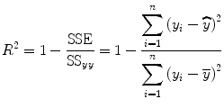
${R}^2=1-\frac{\mathrm{SS}\mathrm{E}}{{\mathrm{SS}}_{yy}}=1-\frac{{\displaystyle \sum_{i=1}^n{\left({y}_i-\widehat{y}\right)}^2}}{{\displaystyle \sum_{i=1}^n{\left({y}_i-\overline{y}\right)}^2}}$

(1.44)

where n is the total number of time points used in the regression analysis and $\widehat{y}$ and $\overline{y}$ are the estimation and mean value of y, respectively.

One example of linear method fitting (solid curve) is shown in Fig. 1.2. In Fig. 1.2, smoothed curve denotes the fitted result from linear regression method. In the figure title, t ₀ is the tracer arrival time and t _eis the tracer first passage ending time; we set t _e ≥ 30% of the maximum concentration after t _max, where t _max is the peak of the concentration–time curve. We only used the concentration time point between t ₀ and t _efor gamma-variate fitting. FWHM denotes full width at half maximum (FWHM) of the gamma-variate function.

1.2.2 Nonlinear Regression Method for Gamma-Variate Fitting

Although linear method has a simple form and easy to program and faster to implement, it is based on the assumption that the model error is homoscedasticity. However, this assumption sometimes does not hold for the data from DSC-MRI; this can lead to large estimation error [24]. Moreover, we cannot estimate tracer arrival time t ₀ using linear regression method. To overcome these shortcomings, nonlinear regression method should be applied [25]. In the literature of nonlinear regression, Gauss–Newton method, steepest descent method, and Levenberg–Marquardt (LM) algorithm are commonly in use. In this section, we provide the details for nonlinear regression using LM algorithm [26]. We define a fit error objective function as

$\begin{aligned}[b] E\left(t,X\right)&=E\left(t;{t}_0,K,\alpha, \beta \right)=\frac{1}{2}{\left[C(t)-K{\left(t-{t}_0\right)}^{\alpha } \exp \left(-\frac{t-{t}_0}{\beta}\right)\right]}^2\\ &=\frac{1}{2}{\left[C(t)-f(t)\right]}^2 \end{aligned}$

(1.45)

where X = [t ₀,K,α,β] is the parameter vector needed to be optimized. To minimize the objective function, we need to calculate a score function $S=\frac{\partial E}{\partial X}$ and then set it to 0, i.e.,

$S=\frac{\partial E}{\partial X}=-{\frac{\partial f}{\partial X}}^{\mathrm{T}}\left[C(t)-K{\left(t-{t}_0\right)}^{\alpha } \exp \left(-\frac{t-{t}_0}{\beta}\right)\right]=0$