(8.1)
where α 2p is a 2p fluorescence coefficient, and I 2p and I ex are, respectively, the intensity of the incident and the fluorescence light at the focal region. Because of the nonlinear process, the implementation of (8.1) in the Monte Carlo simulation model under 2p excitation is not as straightforward as that under 1p excitation. The execution of the Monte Carlo simulation for 2p excitation is divided into two stages. In the first stage, the intensity distribution of the excitation light at the focal plane, I ex(r), where r is the radial coordinate, is calculated and stored in the database. In the second stage, the simulation starts at the focal plane, and fluorescence photons are generated by a uniform random generator. However, the weighting factor for a fluorescence photon at a distance r is determined according to the square of the local intensity of excitation light:
(8.2)
When scattering is strong in a turbid medium, the illumination light distributed outside the focal region becomes more significant, which weakens the optical sectioning property of a 2p fluorescence microscope. Recent experimental research [5, 6] has demonstrated this phenomenon and an approximate theoretical model, which is based on the attenuation of ballistic light by scattering, has been developed to estimate the three-dimensional (3-D) fluorescence intensity distribution in a turbid medium under 2p excitation [7, 8]. The 3-D fluorescence intensity distribution is important to study 3-D image formation in turbid media. However, ignoring the scattered component that is usually stronger than the ballistic component may lead to significant discrepancies in predicting such a 3-D spatial distribution. To overcome this problem, we use the Monte Carlo simulation method to study 1p and 2p fluorescence imaging under a microscope with a particular interest in their 3-D fluorescence light distribution [9].
Here we use a simple approach to extend this model to study the 3-D fluorescence intensity distribution within a turbid medium. First, a stack of planes is identified within a sample volume. By recording the number of photons and their transverse locations where they pass through a given plane, a two-dimensional (2-D) transverse excitation intensity distribution I ex(x, y) can be obtained. Then combining all the 2-D intensity distributions from the stack of planes results in a 3-D excitation intensity distribution I ex(x, y, z). Unlike the model described in [9], which only considers the contribution of fluorescence excitation by ballistic light, the approach used here takes the contribution of fluorescence excitation by both ballistic and scattered photons into consideration. This treatment becomes possible because the Monte Carlo simulation method predicts the behavior of scattered photons as well as ballistic photons.
Consider a turbid medium, illuminated by an objective of numerical aperture (NA) 0.25, and assume that the geometric focal plane is 600 μm beneath the surface. The turbid medium consists of polystyrene beads (reflective index n i = 1.59) suspended in a fluorescence solution such as Rhodamine 590 Tetrafluoroborate dye solution. We assume the illumination wavelength for 1p and 2p excitation is 0.532 and 1.064 μm respectively. Polystyrene beads have a diameter of 0.304 μm, and its corresponding anisotropy values g is 0.25 and 0.72, according to Mie scattering theory , for illumination wavelengths 1.064 and 0.532 μm respectively. The most significant advantage of using 2p excitation instead of 1p excitation is that the illumination wavelength used in 2p excitation is much longer, which results in a smaller scattering cross-section σ s. For a spherical scattering particle (n i = 1.59) of diameter 0.304 μm suspended in water (n i = 1.33), the scattering cross-section σ s is 0.0042 and 0.026 μm2, respectively, for illumination wavelengths 1.064 and 0.532 μm. For a given turbid medium, the scattering-mean-free-path-length (SMFPL) under 2p excitation is more than six times longer than that under 1p excitation.
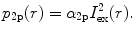
The 3-D fluorescence intensity distribution for 1p excitation I 1p(x, y, z) is shown in Fig. 8.1. Notice that the emission of fluorescence light is limited in the focal region when scattering is weak in a turbid medium (Fig. 8.1a). However, when the turbid medium becomes denser, the amount of fluorescence light excited outside the focal region becomes more significant (Fig. 8.1b, c). It is also seen that the maximum intensity point in I 1p(x, y, z) may shift from the geometric focal region toward the sample surface if the ballistic component in the focal region is negligible (Fig. 8.1d). To explain the features demonstrated in Fig. 8.1, we need to understand the property of two components of photons, the ballistic photon component and the scattered photon component, in the propagation of an illumination beam through a turbid medium. The distribution of ballistic photons depends on the distance between the observation plane and focal plane; the closer the observation plane to the focal region, the narrower the distribution may be formed. Due to the multiple scattering effect, scattered photons deviate from the ballistic path and form a broader distribution in a turbid medium. The ballistic component is dominant in the region close to the sample surface where multiple scattering is insignificant. With the increasing depth into a turbid medium, the scattered component becomes dominant at the focal plane. However, the intensity in the focal region shows a noticeable peak if the turbid medium is not dense (Fig. 8.1a–c), due to the contribution from the ballistic component. Although the total number of ballistic photons is insignificant at a depth of 600 mm, they are concentrated in the focal center, and therefore show a noticeable peak. The ballistic peak becomes weaker when the turbid medium becomes denser, in which situation the total number of ballistic photons becomes negligible (Fig. 8.1d).
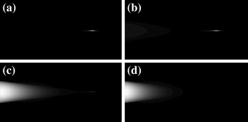
Fig. 8.1
3-D fluorescence intensity distribution I 1p(x, y, z) for 1p excitation (Numerical Aperture = 0.25): a n = 2, b n = 4, c n = 6, d n = 8. Reprinted with permission from [9], 2000, Optical Society of American
The 3-D fluorescence intensity distribution I 2p(x, y, z) for 2p excitation is shown in Fig. 8.2. It should be pointed out that 2p excitation has a much deeper penetration in a given medium due to the fact that longer wavelength illumination light is used. In order to further demonstrate the difference between 1p and 2p excitation, we use the same set of optical thickness in Fig. 8.2. A comparison of Figs. 8.1 and 8.2 shows that for 2p excitation, the fluorescence intensity is significantly stronger in the focal region in relation to the surrounding area (Fig. 8.2a–c) until the scattering is too strong to have a non-negligible ballistic component in the focal region (Fig. 8.2d). The difference between Figs. 8.1 and 8.2 arises from the quadratic intensity dependence in 2p excitation, which efficiently enhances the fluorescence light excited by the ballistic peak in the focal region.
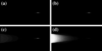
Fig. 8.2
3-D fluorescence intensity distribution I 2p(x, y, z) for 2p excitation (NA = 0.25): a n = 2, b n = 4, c n = 6, d n = 8. Reprinted with permission from [9], 2000, Optical Society of American
To simulate the image of a fluorescence object embedded in turbid media, we introduce an EPSF under 2p excitation. The EPSF is derived from the product of the probability of an excitation photon reaching the focal plane and the probability of a fluorescence photon reaching the detector and the detail of the derivation has been discussed in Chap. 4. The significance of an EPSF is that it enables us to separate the information about an object from a surrounding turbid medium and an imaging system. It is assumed that the excitation and fluorescence wavelengths are 800 and 400 nm, respectively, under 2p excitation. The scattering medium consists of either spherical particles of diameter (ρ) 0.48 μm or spherical particles of diameter 0.202 μm, suspended in water. We assume that the particle concentration in the turbid medium consisting of 0.48 μm particles is 0.87 × 10⁹/mm3. According to Mie Scattering theory, the corresponding SMFPL is 3.68 and 15 μm, respectively, for wavelengths 400 and 800 nm. The optical thickness n is defined as the sample thickness d divided by the SMFPL. For example, if a sample is embedded at a depth of 30 μm, the corresponding optical thickness is 8.14 for wavelength 400 nm. In order to demonstrate the effect of particle size, the SMFPL in a turbid medium consisting of 0.202 μm particles is also assumed to be 3.68 and 15 μm, respectively, for wavelengths 400 and 800 nm. The parameters associated with the two turbid media are summarized in Table 8.1.
Table 8.1
Parameters associated with scattering media
ρ (μm) | λ = 400 nm | λ = 800 nm | ||
|---|---|---|---|---|
g | SMFPL (μm) | g | SMFPL (μm) | |
0.48 | 0.89 | 3.68 | 0.73 | 15 |
0.202 | 0.69 | 3.68 | 0.2 | 15 |
The EPSF for 2p fluorescence imaging is shown in Fig. 8.3. It is seen that a peak is shown near the focal center. With increasing the focal depth, the peak becomes less significant and may eventually disappear if the scattering medium is thick enough. The peak is contributed by the fluorescence light excited by ballistic photons that experience no scattering event on their way to the focal plane. The total number of these ballistic photons may be insignificant compared with scattered photons; however, their contribution to the intensity near focal region may still be significant, since these ballistic photons are only distributed near the focal region. Their contribution to the intensity is enhanced due to the quadratic intensity dependence under 2p excitation. If a photon experiences some scattering events , it deviates from the path of ballistic photon and forms a broad distribution on the focal plane.
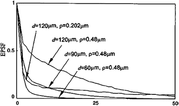
Fig. 8.3
EPSF for 2p fluorescence imaging at different depths d for scatterers of diameters 0.48 and 0.202 mm, respectively, ( , NA = 0.25). Reprinted with permission from [10], 2000, American Institution of Physics
, NA = 0.25). Reprinted with permission from [10], 2000, American Institution of PhysicsThe EPSF at a depth of 120 μm in a turbid medium consisting of 0.202 μm particles is also illustrated in Fig. 8.3. The EPSF has a stronger central peak, but is more widely distributed in this case, compared with the EPSF at the same depth in a turbid medium consisting of 0.48 μm particles. It is understood that the anisotropy value g is less for smaller scattering particles, which results in a broader distribution of the scattered photons in the EPSF. As a result of this property, the intensity outside the focal region is relatively low in a turbid medium consisting of small scattering particles. Therefore, the central peak becomes more significant due to the quadratic intensity response under 2p excitation.
8.1.2 Image Resolution
The transverse resolution of an edge object embedded in a turbid medium consisting of either 0.48 μm particles or 0.202 μm particles is illustrated in Fig. 8.4. It is demonstrated in Fig. 8.4 that 2p fluorescence imaging is vastly superior to 1p fluorescence imaging in terms of image resolution if the depth is less than 60 μm. For 2p fluorescence imaging, the transverse resolution stays nearly at the diffraction-limited resolution when d < 60 μm, and then quickly deteriorates. The deterioration rate eventually drops approximately after d = 90 μm. When d < 60 μm, the fluorescence light excited by ballistic light is dominant over that excited by scattered light, and therefore a near-diffraction-limited image resolution can be achieved. In the range of 60 μm < d < 90 μm, the weighting of the fluorescence light excited by ballistic photons drops quickly and the fluorescence light excited by scattered photons becomes strong, thus leading to poor transverse resolution. In this region, the deterioration rate of transverse resolution depends on the decaying rate of ballistic photons. When d > 90 μm, the scattered component in the EPSF is dominant in building an image. In this situation, the transverse resolution is decided by the broadness of the EPSF contributed by scattered photons.
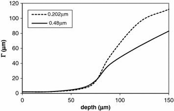
Fig. 8.4
Transverse resolution of a thin edge image as a function of the focal depth for different sizes of scattering particles in 2p fluorescence imaging ( , NA = 0.25). Reprinted with permission from [10], 2000, American Institution of Physics
, NA = 0.25). Reprinted with permission from [10], 2000, American Institution of PhysicsA comparison of the two image resolution curves in Fig. 8.4 shows that the transverse resolution in a turbid medium consisting of 0.48 μm particles is better only when d > 75 μm, in which case scattered photons dominate the imaging process. In the region d < 75 μm, where the central peak in the EPSF dominates the image formation, the resolution is almost the same for the two turbid media.
8.1.3 Signal Level
A comparison of the signal level as a function of the focal depth for 1p and 2p fluorescence imaging is shown in Fig. 8.5. It is shown in Fig. 8.5 that the signal level under 2p excitation drops significantly when the focal depth increases. For example, the signal level drops to only 3 % at d = 30 μm. The signal level for 2p fluorescence imaging decreases faster, compared with the signal level for 1p fluorescence imaging. It is also noticed that the signal level under 2p excitation is more than three orders of magnitude smaller than that under 1p excitation when d = 60 μm. In this situation, the 2p fluorescence signal may be too weak to overcome a noise level from an imaging system. Interestingly, the 2p fluorescence light excited by ballistic photons is still dominant and a near-diffraction-limited resolution can still be obtained at d = 60 μm. Therefore, we may draw the conclusion that 2p fluorescence imaging is mainly determined by ballistic photons, and that the penetration depth is limited by the signal level.
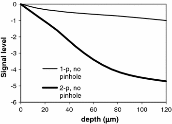
Fig. 8.5
Signal level as a function of the focal depth for 1p and 2p fluorescence imaging, (NA = 0.25, ρ = 0.48 μm). Reprinted with permission from [10], 2000, American Institution of Physics
8.1.4 Penetration Depth
To demonstrate the limiting factor on the penetration depth under 2p and 1p excitation, we consider a turbid medium consisting of scattering particles (diameter 0.202 μm) suspended in water. The turbid medium was placed in a glass cell with lateral dimensions of 2 cm × 1 cm. The thickness of the glass cell, d, was varied from 25 up to 250 μm.
A uniform fluorescent polymer bar was embedded at the bottom wall of the glass cell. The fluorescent bar can be excited under 1p (λ s = 488 nm) and 2p (λ t = 800 nm) excitation to give a peak fluorescence wavelength of approximately 520 nm. Due to the different wavelengths associated with 1p excitation, 2p excitation, and fluorescence the scattering cross-section σ s, the SMFPL l s and the anisotropy value g are different and can be calculated using Mie scattering theory [14] (Table 8.2).
Table 8.2
Calculated values of the scattering cross-section σ s, the scattering mean free path length l s, and the anisotropy value g for polystyrene beads of diameter 0.202 μm at wavelengths 488, 520, and 800 nm, respectively, for a given particle weight concentration of 2.5 %
Wavelength (nm) | Relative particle size, A (a/λ) | Scattering efficiency, Q s = σ s /σ g | Scattering cross-section, σ s (μm2) | SMFPL, l s (μm) | Anisotropy value, g |
|---|---|---|---|---|---|
488 | 0.2069 | 0.1586 | 5.07 × 10⁻³ | 35.7 | 0.54 |
520 | 0.1942 | 0.1356 | 4.34 × 10⁻³ | 41.8 | 0.482 |
800 | 0.1263 | 0.0389 | 1.24 × 10⁻³ | 145.38 | 0.20 |
The prepared sample cell was placed under an Olympus confocal scanning microscope: Fluoview. For 1p excitation, an Ar ion laser at wavelength 488 nm was used. A Spectra-Physics ultrashort pulsed laser: Tsunami, which had a pulse width of 80 fs, was employed for 2p excitation at wavelength 800 nm. To avoid the effect of the refractive-index mismatching between the turbid medium and the cover glass of the cell, a water-immersion objective (Olympus UplanApo 60×, ∞/1.13–0.21, NA = 1.2, working distance = 250 μm) was used. In the case of 1p excitation, a pinhole of 300 μm in diameter was placed in front of the detector to produce an optical sectioning effect with strength similar to that under 2p excitation without using pinhole. The dependence of the signal level and the resolution α on the cell thickness d is depicted in Figs. 8.6 and 8.7 which also includes the Monte Carlo simulation results corresponding to the experimental condition. A good agreement between experiments and theoretical predictions is observed. For the turbid medium we used, the image resolution under 2p excitation is two orders of magnitude higher than that under 1p excitation, while the signal strength attenuates much faster with increasing depth.
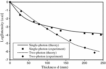
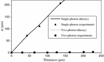
Fig. 8.6
Signal level under 2p and 1p excitation as a function of the penetration depth of a turbid medium consisting of scatterers of diameter 0.202 μm. Reprinted with permission from [11], 2000, American Institution of Physics
Fig. 8.7
Image resolution under 2p and 1p excitation as a function of the penetration depth of a turbid medium consisting of scatterers of diameter 0.202 μm. Reprinted with permission from [11], 2000, American Institution of Physics
Although the above results were obtained for a given size of scatterers, the conclusion regarding the effect of Mie scatterers on 2p excitation holds for other sized Mie scatterers. In particular, the smaller the scatterer size, the smaller the anisotropy value and the larger the SMFPL. Based on this property, we can conclude that for a real tissue medium consisting of different size of Mie scatterers, the 2p fluorescence signal level is lower than 1p signal level at a deep depth. This conclusion is demonstrated in Figs. 8.8 and 8.9. The penetration depth of 2p excitation in imaging through a tissue medium is smaller than that of 1p excitation because of the lower signal level in the former case. However, within the depth of detectable signal, 2p excitation leads to image resolution significantly higher than that under 1p excitation.
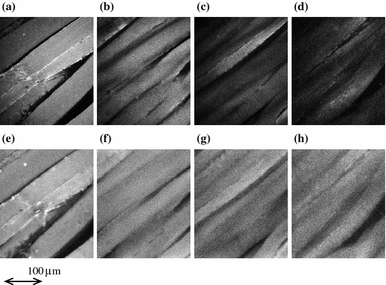
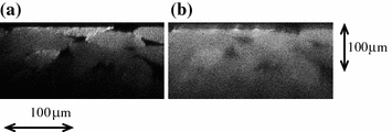
Fig. 8.8
Measured transverse (x–y) images through a thick muscle tissue sample under 2p and 1p excitation. a–d 2p fluorescence images at depths of 10, 30, 50, 70 μm; e–h 1p fluorescence images at depths of 10, 30, 50, 70 μm. Reprinted with permission from [11], 2000, American Institution of Physics
Fig. 8.9
Measured axial (x–z) images through a thick muscle tissue sample under 2p (a) and 1p (b) excitation. Reprinted with permission from [11], 2000, American Institution of Physics
8.2 Influence of System Parameters
Commonly, the performance of an imaging system is governed by the point spread function which is determined by system parameters such as the NA of the objective lens, the size of a confocal pinhole, etc. In this section, the influence of various parameters associated with a microscopic imaging system under the 2p excitation is discussed in detail.
8.2.1 Numerical Aperture
For the same scattering media described in Sects. 8.1.1–8.1.3, the EPSF at a depth of 120 μm for 2p fluorescence imaging is shown in Fig. 8.10 for different values of the NA of an objective. The EPSF for 2p excitation is not necessarily poorer if a higher NA objective is used. In fact, in this situation, the central peak is more pronounced, but the EPSF appears to be broader.
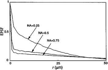
Fig. 8.10
EPSF for different values of the numerical aperture of an objective in 2p fluorescence imaging ( , ρ = 0.48 μm). Reprinted with permission from [10], 2000, American Institution of Physics
, ρ = 0.48 μm). Reprinted with permission from [10], 2000, American Institution of PhysicsIn Fig. 8.11, the transverse resolution as a function of the focal depth is illustrated for different values of the NA of an objective. It is noted that for d < 60 μm, the image resolution is slightly better if a higher Na objective is used. In this region, the central peak in the EPSF is dominant in forming an image. The central peak in the EPSF is mainly contributed by fluorescence excited by ballistic photons. Therefore, a near-diffraction-limited resolution can be achieved in this situation. Since a higher NA objective produces a narrower diffraction spot, the corresponding transverse resolution is better. In the region where d > 90 μm, the transverse resolution is better when a lower NA objective is used. In this region, the broad distribution in the EPSF, contributed by scattered photons, is dominant in image formation. In this situation, a high NA objective collects more scattered photons, which results in a broader distribution in the EPSF, and therefore leads to poorer resolution. It is in the region of 60 μm < d < 90 μm where the central peak in the EPSF starts to lose its dominance that a quicker degradation in image resolution occurs for a higher NA objective.
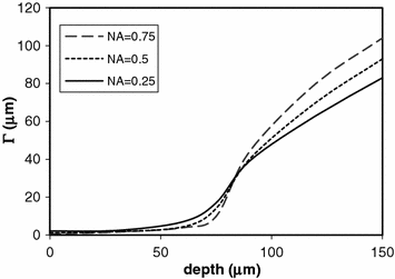
Fig. 8.11
Transverse resolution for different values of the NA of an objective in 2p fluorescence imaging ( , ρ = 0.48 μm). Reprinted with permission from [10], 2000, American Institution of Physics
, ρ = 0.48 μm). Reprinted with permission from [10], 2000, American Institution of PhysicsIn conclusion, when the ballistic peak in the EPSF is dominant in forming an image, a higher NA objective offers a better resolution. When the broad distribution contributed by scattered photons is dominant, a lower NA objective gives better transverse resolution.
8.2.2 Confocal Pinhole
Now we consider the effect of a pinhole on 2p fluorescence imaging. It has been demonstrated in Chap. 7 that a confocal pinhole is efficient in suppressing highly scattered photons, and as a result, it provides a significant improvement in the 1p fluorescence imaging. The EPSF for a pinhole of diameter 100 μm at a depth of 120 μm is illustrated in Fig. 8.12a. It is noted that the utilization of a finite sized pinhole makes little difference in the central peak of the EPSF. However, it does reduce the contribution of scattered photons in the region outside the focal center. This feature implies that a pinhole may not be efficient in improving image quality in 2p fluorescence imaging through turbid media if the central peak is dominant in the EPSF. In Fig. 8.12b, the transverse resolution as a function of the focal depth is illustrated. As expected, the resolution improvement by utilization of a finite sized pinhole is not significant until a turbid medium becomes thicker, d > 75 μm, in which case the fluorescence excited by scattered photons is dominant.
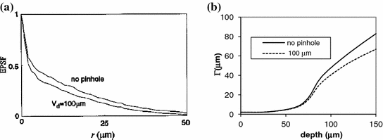
Fig. 8.12
a EPSF foa a pinhole of diameter 100 μm at a depth of 120 μm; b resolution; c signal level for a confocal microscope. Reprinted with permission from [10], 2000, American Institution of Physics
The utilization of a pinhole offers little improvement in 2p fluorescence imaging in terms of image resolution (Fig. 8.12b). Moreover, using a pinhole significantly reduces signal strength (Fig. 8.12c), which can be a serious problem in 2p fluorescence imaging through turbid media. For example, at d = 60 μm, the improvement in transverse resolution is only 9.5 % when a pinhole of diameter 100 μm is used. However, the signal strength drops to only 31 % of the signal level when no pinhole is used. It appears that using a pinhole in 2p fluorescence imaging through turbid media is unwise.
Related posts:
Stay updated, free articles. Join our Telegram channel

Full access? Get Clinical Tree


