be m (m = 39) members of the aligned training surface models. Each member is described by a vector Xi with N (N = 5000) vertices:

(1)
A PDM was then obtained by applying principal component analysis [24] to the aligned training surface models:

where  and
and  are the mean vector and the covariance matrix of the PDM, respectively.
  are non-zero eigenvalues of the covariance matrix
  , and
, and  are the corresponding eigenvectors. The descendingly sorted eigenvalues
  and the corresponding eigenvector
  are the principal directions spanning a shape space with
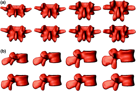
  representing its origin. Figure 1 shows the variability captured by the first two modes of variations of the PDM.

(2)
 and
and  are the mean vector and the covariance matrix of the PDM, respectively.
  are non-zero eigenvalues of the covariance matrix
  , and
, and  are the corresponding eigenvectors. The descendingly sorted eigenvalues
  and the corresponding eigenvector
  are the principal directions spanning a shape space with
  representing its origin. Figure 1 shows the variability captured by the first two modes of variations of the PDM.
Fig. 1
The first two principal modes of variation of the PDM used in this investigation. The shape instances from left to right at each row were generated by evaluating 
 with (a) Posterior view of the PDM (k = 1: the 1st row; k = 2: the 2nd row); and (b) Lateral view of the PDM (k = 1: the 1st row; k = 2: the 2nd row)

 with (a) Posterior view of the PDM (k = 1: the 1st row; k = 2: the 2nd row); and (b) Lateral view of the PDM (k = 1: the 1st row; k = 2: the 2nd row)
3 Statistically Deformable 2D/3D Reconstruction
Without loss of generality, here we assume that the input image is calibrated and image distortion is corrected. For more details about fluoroscopic image calibration, we refer to our previous work [25]. Thus, for a pixel in the input image we can always find a projection ray emitting from the focal point of the image through the pixel.
The single image based surface model reconstruction technique proposed in this paper is based on a hybrid 2D/3D deformable registration process coupling a landmark-based scaled rigid registration with an adapted SSM-based 2D/3D reconstruction algorithm [20, 21]. Different from the situation in our previous works [20, 21], where two or more calibrated X-ray images were required as the input for a successful reconstruction, here only a single lateral fluoroscopic image is available. Similar to the situation when multiple images are used, the convergence of the single image based 2D/3D reconstruction also depends on the initialization and on the image contour extraction. Thus, in the following we focus on the image contour extraction and on a landmark-based scaled rigid registration for initializing the single image based 2D/3D reconstruction.
3.1 Image Contour Extraction
As a feature-based 2D/3D reconstruction approach, our technique requires a pre-requisite image contour extraction. Explicit and accurate contour extraction is a challenging task, especially when the shapes involved become complex or when the background of the image becomes complex. In this paper, we feel that it is a far better choice to provide the user with a tool that supports interactive segmentation but at the same time speeds up the tedious manual segmentation process and makes the results repeatable. This leads us to developing a semi-automatic segmentation tool.
Our semi-automatic segmentation tool is based on the Livewire algorithm introduced by Mortensen and Barrett [26]. In their paper, graph edges are defined as the connection of two 8-adjacent image pixels. A local cost function is assigned to the graph edges to weight their probability of being included in an optimal path. In this work, we use two static feature components to form this cost function. The first component  is calculated from Canny edge detectors [27] at three different scales (the standard deviations of the Gaussian smoothing operator in these three scales are 1.0, 2.0, and 3.0, respectively) as follows.
 is calculated from Canny edge detectors [27] at three different scales (the standard deviations of the Gaussian smoothing operator in these three scales are 1.0, 2.0, and 3.0, respectively) as follows.
Let’s denote the edges extracted by the Canny edge detector at three different scales as  ,
,  , and
, and  , respectively.
  are defined as follows: if pixel
  is a detected edge pixel at the ith scale, then
  ; otherwise, it equals to zero. Let’s further denote the gradient magnitudes at different scales as
  ,
,  , and
, and  , respectively. Then we have,

 ,
,  , and
, and  , respectively.
  are defined as follows: if pixel
  is a detected edge pixel at the ith scale, then
  ; otherwise, it equals to zero. Let’s further denote the gradient magnitudes at different scales as
  ,
,  , and
, and  , respectively. Then we have,
(3)
According to Eq. (3), if  is not a detected edge pixel at the ith scale, a constant cost of 1.0 will be added to the cost function. Otherwise, the cost depends on the gradient magnitude: the bigger the magnitude, the smaller the cost.
 is not a detected edge pixel at the ith scale, a constant cost of 1.0 will be added to the cost function. Otherwise, the cost depends on the gradient magnitude: the bigger the magnitude, the smaller the cost.
The second component, the gradient direction  , is calculated according to the form proposed in the original paper [26], which is used to add a smoothness term to the contour definition by assigning high costs to sharp changes.
 , is calculated according to the form proposed in the original paper [26], which is used to add a smoothness term to the contour definition by assigning high costs to sharp changes.
Finally, these two static features are combined by weighted summation to form a single statistic local cost function as follows

where the weights for these two terms are empirically determined.

(4)
Based on the Livewire algorithm, the semi-automatic contour extraction starts with a seed point, which is interactively placed by the user with a click of the left mouse button. During the extraction, the user can add more seed points by clicking the left mouse button. A click of the right mouse button will finish the definition of one contour. After that, clicking the left mouse button again starts the extraction of a new contour. Figure 2 shows an example of how the livewire segmentation technique is used to extract contours from the input image.
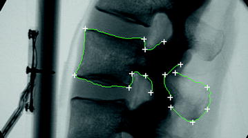

Fig. 2
Example of using livewire segmentation algorithm to extract image contours. The white crosses show where the user clicks the mouse button
3.2 Landmark-Based Scaled Rigid Registration for Initialization
Initialization here means to estimate the initial scale and the rigid transformation between the mean model of the PDM and the input fluoroscopic image. For this purpose, we have adopted an iterative landmark-to-ray scaled rigid registration. The four anatomical landmarks that we used here are the center of the top surface of the vertebra body, the center of the bottom surface of the vertebra body, the geometrical center of the vertebra body, and the center of the spinal process tip. Their positions on the mean model of the PDM are obtained through point picking or center calculation (the center of the vertebra body is computed as the center of four boundary landmarks along the anterior-posterior direction as shown in Fig. 3a, while their positions on the fluoroscopic image are defined through interactive picking (see Fig. 3a, b for details).
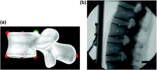

Fig. 3
Definition of initialization landmarks. a Landmarks extracted from the mean model of the PDM. b Landmarks extracted from the fluoroscopic images
Let us denote those landmarks defined on the mean model of the PDM, i.e., the vertebra body center, the center of the top surface of the vertebra body, the center of the bottom surface of the vertebra body and the center of the spinal process tip, as  ,
,  ,
,  , and
, and  , respectively; and their corresponding landmarks interactively picked from the fluoroscopic image as
  ,
,  ,
,  , and
, and  , respectively. And for each X-ray landmark, we can calculate a projection ray emitting from the focal point to the landmark. We then calculate the length between
  and
and  and denote it as
  . Using the known image scale, we also calculate the length
  between
  and
and  . Then, we do:
 ,
,  ,
,  , and
, and  , respectively; and their corresponding landmarks interactively picked from the fluoroscopic image as
  ,
,  ,
,  , and
, and  , respectively. And for each X-ray landmark, we can calculate a projection ray emitting from the focal point to the landmark. We then calculate the length between
  and
and  and denote it as
  . Using the known image scale, we also calculate the length
  between
  and
and  . Then, we do:
Data Preparation. In this step, we assume that the line connecting the centers of the vertebra body and the center of the spinal process tip is parallel to the input fluoroscopic image and is certain distance away from the imaging plane. Using this assumption and the correspondences between the landmarks defined in the CT volume and those from the fluoroscopic image, we can compute two points  and
and  on the projection rays of
  and
and  , respectively (see Fig. 4a), which satisfy:
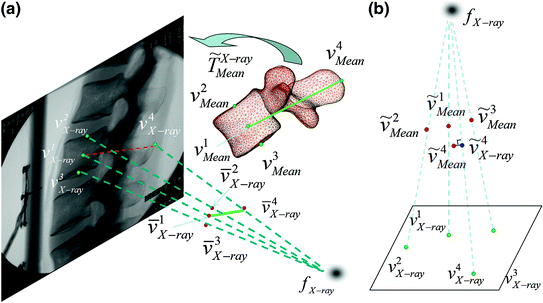

where “//” symbol indicates that the two lines are parallel;  is the calibrated distance from the focal point to the imaging plane and
  is the assuming distance from the line connecting the center of the vertebra body and the center of the spinal process tip to the imaging plane.
 and
and  on the projection rays of
  and
and  , respectively (see Fig. 4a), which satisfy:
Fig. 4
Iterative landmark-to-ray registration. a Schematic view of data preparation. b Schematic view of finding 3D point pairs

(3)
 is the calibrated distance from the focal point to the imaging plane and
  is the assuming distance from the line connecting the center of the vertebra body and the center of the spinal process tip to the imaging plane.
The current scale s between the mean model and the input image is then estimated as,


(4)
Using s, we scale all landmark positions on the mean model and denote them as  . We then calculate the distances from
  and
and  to the line
  and denote it as
  and
and  , respectively.
 . We then calculate the distances from
  and
and  to the line
  and denote it as
  and
and  , respectively.
Next we find two points, point  on the projection ray of
  whose distance to the line
  is equal to
  , and point
  on the projection ray of
  whose distance to the line
  is equal to
  . A paired-point matching based on
  and
and  is used to calculate an updated scale
  and a rigid transformation
  (see Fig. 4a for details). From now on, we assume that all information defined in the mean model coordinate frame has been transformed into the fluoroscopic image coordinate frame using
  and
and  . We denote the transformed mean model landmarks as
  .
.
 on the projection ray of
  whose distance to the line
  is equal to
  , and point
  on the projection ray of
  whose distance to the line
  is equal to
  . A paired-point matching based on
  and
and  is used to calculate an updated scale
  and a rigid transformation
  (see Fig. 4a for details). From now on, we assume that all information defined in the mean model coordinate frame has been transformed into the fluoroscopic image coordinate frame using
  and
and  . We denote the transformed mean model landmarks as
  .
.Stay updated, free articles. Join our Telegram channel

Full access? Get Clinical Tree


