CHAPTER 79 Physics of Computed Tomography
FUNDAMENTALS OF X-RAY PHYSICS
In the diagnostic x-ray energy range between 20 keV and 140 keV, there are three types of interactions between x-ray photons and the patient: photoelectric effect, Compton scatter, and coherent scatter.1–3 In photoelectric interaction, the incident x-ray photon energy is greater than the binding energy of a deep shell electron. By giving up its entire energy in liberating the electron, the original x-ray photon no longer exists. When the hole created at the deep shell is filled by an outer shell electron, a characteristic radiation is generated. Because the probability of such interaction is proportional to the cube of the atomic number of the matter, tissues with small differences in atomic numbers result in a greater difference in the x-ray photon absorption and lead to greater contrast between different tissues.

where I0 is the intensity of the x-ray beam impinging on a uniform material of thickness Δx, I is the x-ray intensity after passing through the material, and µ is the linear attenuation coefficient of the material; µ changes with the input x-ray energy and varies for different materials. Figure 79-1 shows, on a logarithmic scale, µ as a function of energy for soft tissue (red), cortical bone (green), and iodine (blue). It is clear from the figure that significant difference exists between the attenuation coefficients for the three materials, and iodine is more attenuating to the x-ray photons than the bone, which in turn is more attenuating than the soft tissue. As a result, when iodine-based contrast material is injected intravenously into the patient and imaged under x-ray examination, blood vessels generate stronger attenuating signals and therefore become more visible over the diagnostic x-ray energy range.
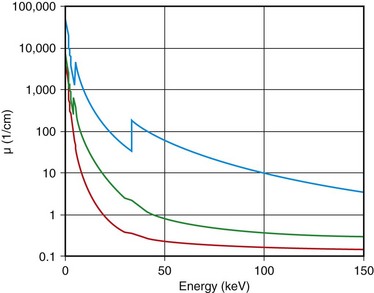
 FIGURE 79-1 Linear attenuation coefficients as a function of energy: red, soft tissue; green, bone; blue, iodine.
The x-ray photons produced by the x-ray tube on all clinical x-ray devices today have a wide energy spectrum. For example, when 120 kVp is prescribed on an x-ray CT scanner, x-ray energies ranging from 20 keV to 120 keV are emitted. Because the amount of attenuation to these x-ray photons varies significantly, even for a single material as demonstrated in Figure 79-1, the measured attenuation of an object is consequently the averaged effects of different energy x-ray photons weighted by their spectrum.
IMPORTANT PERFORMANCE PARAMETERS OF X-RAY COMPUTED TOMOGRAPHY
There are many parameters that define the performance of a CT scanner.1,4–6 During the system design, conscious decisions have to be made to trade off some performance parameters against others to optimize the overall performance for a particular application. In this section, a few important performance parameters of the CT system are discussed, and it should be understood that this is by no means a complete list.
Spatial resolution defines the ability of a CT scanner to resolve closely spaced high-contrast objects and is often specified in terms of line pairs per centimeter (lp/cm). A pattern of 1 lp/cm is formed by a pair of high- and low-intensity bars, each 5 mm in width, as shown in Figure 79-2A; a pattern of 4 lp/cm contains four such high- and low-intensity bars within each centimeter space, as depicted in Figure 79-2B. It is clear from the figure that as the width of the bars is reduced and the bars are closely packed together, it becomes increasingly difficult for a CT system to resolve or to identify the bars individually. To measure the spatial resolution of a CT system, standard bar phantoms are scanned and reconstructed. An example of such a phantom (Catphan) is shown in Figure 79-3. In this phantom, bar patterns of different frequencies are positioned at a fixed radius from the phantom center, and system response to these frequencies can be evaluated from a single scan.
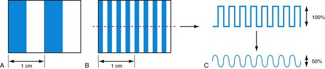
 FIGURE 79-2
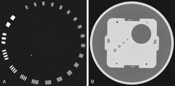
 FIGURE 79-3 Reconstructed images of resolution phantoms. A, Catphan. B, GE Performance phantom.
(B courtesy of GE Healthcare Technologies, Waukesha, Wisc.)
To quantitatively describe the spatial resolution performance, modulation transfer function (MTF) is typically employed. If we plot the profile of the original 4 lp/cm bar pattern object, we obtain a set of rectangular functions as shown by the upper portion of Figure 79-3C. In a similar fashion, we can plot the profile of the reconstructed image of the same bar pattern and obtain a smoothed version of the original rectangular pattern shown by the lower portion of Figure 79-2C. Because of the limited frequency response of the system, both the sharpness and the peak-to-valley magnitude of the reconstructed bar pattern are reduced compared with the original. In the example shown, the magnitude of the reconstructed object is only 50% of the original. Therefore, the MTF value at 4 lp/cm for this system is 0.5. By plotting the peak-to-valley magnitude over different frequencies, a complete MTF curve is obtained. The MTF accurately describes a system’s frequency response and is a good indicator of the system’s ability to resolve small objects. Alternatively, MTF curves can be obtained from the reconstructed phantom image of a thin wire, based on the fact that MTF is the magnitude of the Fourier transform of the point-spread function. Figure 79-3B shows a reconstructed image of a GE Performance phantom, and the wire section of the image is extracted to generate the MTF curve.
The importance of spatial resolution can be easily understood because it is an indicator of how well a small structure can be visualized. For example, Figure 79-4 depicts a volume rendered image of a CT angiography scan collected on a multislice CT scanner. High spatial resolution enables the clear visualization of small vascular structures. Another example is depicted in Figure 79-5 of two volume rendered images of a stent. Clear visualization of the stent allows the evaluation and assessment of its integrity or potential of restenosis in many clinical applications. Figure 79-5A was obtained on a multislice CT scanner; Figure 79-5B was obtained on a high-definition scanner. Because of the increased spatial resolution offered by the high-definition scanner, the stent structure is better visualized.
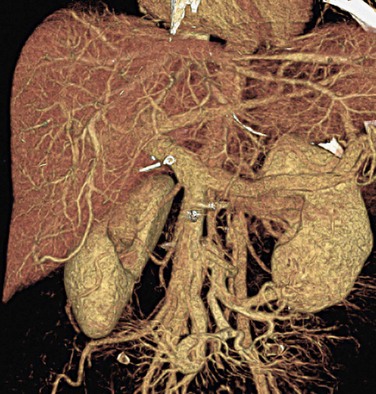
 FIGURE 79-4
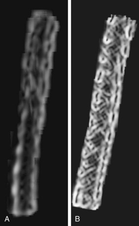
 FIGURE 79-5 Volume rendered images of a 3-mm stent. A, The multislice CT image. B, High-definition image.
(Courtesy of GE Healthcare Technologies, Waukesha, Wisc.)
where µ is the linear attenuation coefficient of the object of interest and µw
Stay updated, free articles. Join our Telegram channel

Full access? Get Clinical Tree


