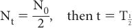
, known as the half-life. This is defined as the time interval for a given number of nuclei (or their radioactivity) to decay to one-half of the original value. For example, if initially there are 10,000 nuclei in a radionuclide and 5000 of them decay in 5 days, then the half-life of this radionuclide is 5 days. Therefore, by definition of the half-life, when
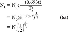
If we substitute these values in equation (3), we obtain
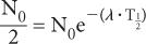
Or
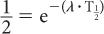
Because e−0.693 is equal to 1/2 (see Appendix C), it follows that

Equation (5) relates the decay constant to the half-life of a radionuclide. From this, if one knows the half-life of the radionuclide, one can calculate the decay constant or vice versa.
Example:
Half-life of 131I = 8 days. Determine the decay constant for 131I
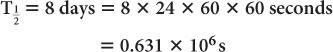
From equation (5),

Problems on Radioactive Decay Equations (1) to (5) are the basic equations necessary for solving routine problems in nuclear medicine. In general, to solve such problems, use of exponential tables is necessary (Appendix C). However, in special cases, where multiples of half-life are involved, equation (3) can be written in a simpler form by substituting the value of from equation (5).
When t is a multiple of  , it is easier to make calculations using the above expression than to use exponential tables. For example, if one is interested in finding the number of radioatoms remaining after an interval t = 3 × the half-life of a radionuclide, the above expression becomes
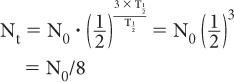
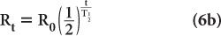
or one-eighth of the original number. A similar simplification occurs for the activity:
Example 1:
A radioactive sample of 99mTc contains 370 MBq (10 mCi) radioactivity at 9:00 a.m. What will be the radioactivity of this sample at 3:00 p.m. on the same day? (The half-life of 99mTc is 6 hours.) In this example,
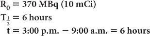
Now, using equation (6b)

Example 2:
A preparation of 99mTc was calibrated at 7 a.m. and contained 555 MBq/mL (15 mCi/mL) of radioactivity at that time. If the prescribed dosage to the patient is 555 MBq (15 mCi), determine the volume of the preparation that will have to be injected at 10 a.m.
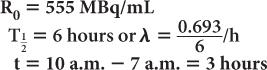
Using equations (4) and (5)
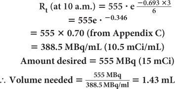
Example 3:
An iodine-123 capsule is calibrated to contain 100 μCi (3.7 MBq) at noon. However, the capsule is given to a patient early in the morning at 9 a.m. Find the dosage of 123I administered to the patient. (Half-life of 123I = 13 hours.)
Let us assume that the radioactivity at 9 a.m. is R0. Then, the radioactivity at noon (i.e., 3 hours later) is Rt = 100 μCi. Using equations (4) and (5), we get
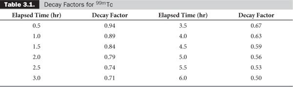
Quite often, the term e-λ·t is tabulated for various intervals of time for a given radionuclide. These are known as decay factors. In example 3, the decay factor for 123I for 3-hour decay is 0.85. If the table of decay factors is available, then the relationship of Rt and R0 becomes simplified as Rt = R0 × decay factor, where decay factor = e−λ·t. Table 3.1 lists some decay factors for 99mTc.
For practical considerations, a simple fact to remember is that the radioactivity remaining after 10 half-lives of a radionuclide is about one-thousandth of the original radioactivity (i.e., MBq amounts are reduced to kBq amounts or millicurie amounts are reduced to microcurie amounts). This is so because (1/2)10 ~ 1/1000.
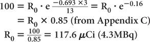
Average Life (Tav) Occasionally, we encounter the use of another term known as average life of a radionuclide. It is related to the half-life of the radionuclide or the decay constant as follows:
Because in radioactive decay not all radioatoms decay at the same time, each individual radioatom exists for a different period of time. Average life is therefore the mean of all these intervals for which individual radioatoms remain in existence.
Biological Half-Life Under many circumstances, the disappearance with time of a biochemical or drug in a biological system (e.g., thyroid, liver, lungs, bone, blood, plasma, or reticuloendothelial cells) can be described by an exponential law similar to that which holds true for radionuclidic decay. In this case, the disappearance of the biochemical or drug is accomplished through metabolism, excretion, simple diffusion, or some other ill-defined bio-mechanism. The amount Mt of the biochemical or drug present in the biological system at time t can be determined by an equation similar to that used to determine radioactivity Rt [equation (4)], provided the original amount M0 of the biochemical or drug and the probability of its disappearance λBio in the biological system under consideration is known. In that case,

The disappearance probability λBio is related to the biological half-life  (Bio), by an equation similar to equation (5):

The biological half-life is defined as the interval during which a given amount of a biochemical or drug in a biological system is reduced to one-half its original value.
Often the disappearance of a biochemical or drug in the biological system cannot be described by equation (7). In these cases, the disappearance of the biochemical or the drug can be described by a sum of several exponential terms as follows:

where A1, A2… and λ1Bio, λ2Bio… are constants and are determined experimentally for a given drug in a given biological system.
Effective Half-Life In nuclear medicine, one is interested in the distribution and the disappearance with time of radioactive substances or drugs from biological systems as a result of both physical decay and biological elimination (metabolism, diffusion, or excretion). Such information is crucial in radiation dose calculations to a patient and to determine the optimum time for imaging after the administration of the radiopharmaceutical.
In the simple case of mono-exponential biological distribution and disappearance [equation (7)], the probability of disappearance of a radiopharmaceutical from a biological system is the sum of both the physical and biological disappearance probabilities, i.e.:

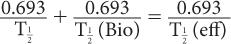
where λeff is the effective disappearance probability for a radioactive substance or drug. If one converts the various disappearance constants in equation (9) to their respective half-lives, equation (9) becomes
or
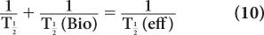
From this relationship [equation (10)], one can determine the effective half-life of a radiopharmaceutical if the physical half-life of the radio-nuclide and the biological half-life of the drug (or chemical) are known. As a rule, however,  (eff) will always be less than or equal to the shorter of the two,
  and
and  (Bio).
In the complex case of biological distribution and disappearance [equation (8a)], it becomes difficult to define a single effective half-life unless each exponential represents a separate biological compartment or organ. Then, each compartment or organ has an effective half-life determined by the physical half-life and the biological half-life for that organ or compartment.
Example:
(1) The biological half-life of iodine in human thyroid is about 64 days, and the physical half-life of 131I is 8 days. Determine the effective half-life of 131I in the thyroid.
Given:

Therefore, from equation (10),
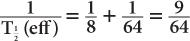
or
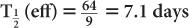
(2) Xenon-133, a radioactive inert gas, is used for lung-function studies. Its physical half-life is 5.3 days and its biological half-life in the lungs is about 0.35 minutes. Determine the effective half-life of 133Xe in the lungs. Given:
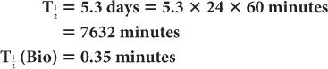
Therefore, from equation (10),
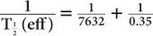
or
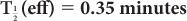
In this example,  (eff) = T
 (Bio). Actually, whenever one of the half-lives,
  or
or  (Bio), is very large (10 times or more) in comparison with the other, then
  (eff) is equal to the other half-life
  (Bio) or
  ). In mathematical terms,

or

Statistics of Radioactive Decay
Although is defined here as the probability of decay per unit time per atom, in earlier discussions it has been tacitly assumed that the number of radioatoms that decay in time t can be accurately determined. This is not so, nor is there any way to predict exactly which particular atom will decay at a given moment. In practice, the number of radioatoms that decay in a given time t fluctuate around an average value, and for this reason the equations described in the preceding sections express only the relationships of the average values of Nt and Rt.
Because of these statistical variations in nuclear measurements, it is essential to know what contribution these fluctuations make to the total error of a measurement. Barring blunders, error in any measurement has two causes, systematic and random. Systematic errors are caused by the use of improperly calibrated instruments and will always either underestimate a measurement or overestimate it, depending on which way the error has been made in calibration. Random errors are caused by some uncontrollable factors. Therefore, when a number of repeat measurements are made, these tend to be randomly distributed. The term “accuracy” is used to describe systematic errors, whereas “precision” is used to describe random errors. In radioactivity measurements, random errors that are the result of the natural decay process dominate over the systematic errors and therefore are taken into account only. I should point out here that this discussion of errors is not limited only to counting but is of importance in imaging as well.
Poisson Distribution, Standard Deviation, and Percent Standard Deviation The probability that a given number of disintegrations N will actually occur in a radioactive sample in time t, when the mean number of dis-integrations for that sample is  is determined by the Poisson distribution. The mathematical or graphic description of Poisson distribution is complicated. Therefore, it is generally approximated with a Gaussian or standard distribution, shown in Figure 3.3. A Gaussian distribution, which is completely determined by two parameters, mean
  and standard deviation σ, is given by the following expression
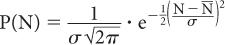
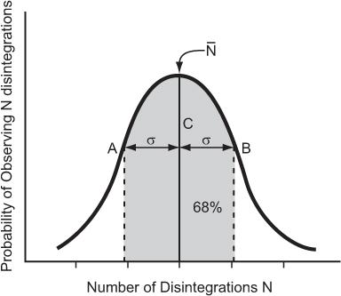
Fig 3.3. Poisson distribution (for large values of N, it is similar to a Gaussian distribution) showing the random nature of radioactivity. The width σ (AC or BC) is known as standard deviation SD. A range of N + σ to N − (A to B) covers about 68% of the total area of the distribution curve.
where P(N) is the probability for observing N disintegrations,  is the average number of dis-integrations, and is the standard deviation SD. SD determines the spread or width of a Gaussian (or Poisson) distribution and is commonly used as a measure of random error, or precision, of a radioactive measurement.
A range of N − σ to N + σ(1 SD) implies that the probability of a given measurement lying within this range is about 68%. When the range is extended to include 2 SDs (N − 2σ to N + 2σ), the probability increases to 95%. Further extension of the range to include 3 SDs (N − 3σN + 3σ) increases the probability to 99%.
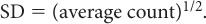
An important characteristic of Poisson distribution is the relation of its SD to the mean number of disintegrations  as follows:
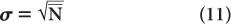
For large values of  , this equation allows a rapid determination of the SD of a given measurement if we replace
  by N.
by N.
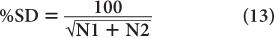
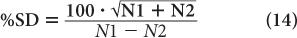
A more useful index of statistical error or precision of a measurement than SD is percent standard deviation % SD. The % SD of a measurement is determined as follows:
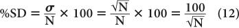
This equation states that the precision of a given radioactive measurement can be increased by increasing the observed number of disintegration. In practical terms, this means that if we measure a radioactive sample for 1 minute and obtain 100 disintegrations during this time, then its % SD, as determined from the above relationship, will be equal to

or 10%. However, if we measure the sample long enough (approximately 100 times longer) so that there are 10,000 disintegrations during this interval, the % SD in this case will be equal to

or 1%. In other words, by increasing the time of counting (approximately 100 times), we have decreased the percent error in our results (only by a factor of 10). When the time of counting is limited, a compromise has to be made between the length of counting time and precision.
Propagation of Statistical Errors In many nuclear applications, we have to add, subtract, multiply, or divide two or more measurements. How does one determine the precision of the final result? To answer this question, let us assume that N1 and N2 are two measurements from which the final result N is obtained by adding, subtracting, dividing, or multiplying N1 and N2. Without going into detail, then, the SD of N is given by the following expressions:
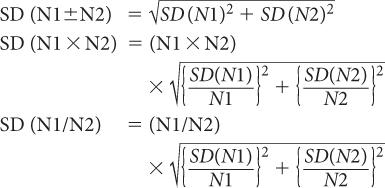
The % SD of N is given by the following expressions:
When adding:
When multiplying or dividing:

Error in Count Rate Count rate R of a sample is determined by dividing the number of counts N observed in a time interval t by the time interval t or
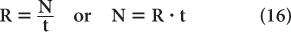
Because the error in the measurement of time t is generally very small, the error in R mainly results from the error in N. Therefore,
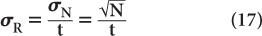
Substituting N = R · t from equation (16), we get
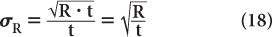
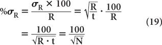
To reduce the error of a count rate R, one has to increase the averaging time t. The % σR of a count rate is given by the following expression:
Room Background Even when there is no radioactive sample near a radiation detector, it will still record a certain number of disintegrations known as room background. This is due to the presence of minute amounts of radioactivity in the surrounding earth and/or building material. Part of the room background is also contributed by the high-energy radiations of cosmic rays. Room background can be reduced to a low level by shielding the radiation detector. However, it cannot be reduced to zero because of the presence of trace amounts of radioactive substances in the detector and shielding materials themselves and because of the inability to completely shield against high-energy background radiation. In situations where the sample count rate is very low (less than ten times of background), it is important to take into consideration the room background and its effect on the precision of the final result.
Examples
(1) In the thyroid uptake measurement of a patient, it is found that the neck activity gives 900 counts per minute, whereas the standard is 2500 counts per minute. Calculate the % uptake by the thyroid and its precision.
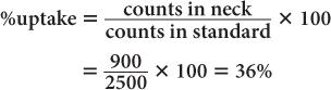
Using equation (12),
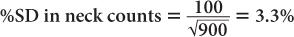
and
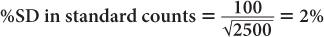
Using equation (15),
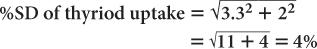
Therefore,
Thyroid uptake = (36 ± 4%)%
Because 4% of 36 is 1.4,
Thyroid uptake = (36 ± 1.4)%
(2) A radioactive sample registers a total (sample + background) of 3200 counts in 1 minute. The room background is 1000 counts per minute. Calculate the net counts of the sample and the % SD of the total counts, background, and the net counts, respectively.
Net counts in the sample
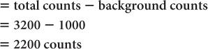
Using equation (12),
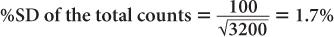
and

Using equation (14),
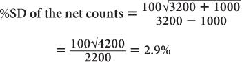
This clearly demonstrates the manner in which the room background degrades the precision of a radioactive measurement.
Key Points
1. Radioactivity of a sample is defined as the rate of decay. Its unit is Bq (1 disintegration/s) in SI units and curie (3.7 × 10¹⁰ disintegration/s) in old units.
2. Radioactivity of a sample at time t, Rt depends on the radioatoms Nt present at that instant and a characteristic decay constant of the radionuclide, and Rt = Nt.
3. Nt and Rt decay with time through law of exponential (i.e., Nt or Rt = N0 or R0e−λt).
4. Half-life of a radionuclide is related to the decay constant, λ as λ
= 0.693.
5. Biological half-life and effective half-life are defined in a similar fashion to physical half-life of a radionuclide for a biochemical and a biochemical labeled with a radionuclide, respectively.
6. Radioactive decay is random and follows Poisson statistics. It is impossible to predict how many decays will occur exactly in a given second or minute.
7. Standard deviation SD is used to measure the range in which such decay may lie. This is used to quantify error of a radioactive measurement.
8. For Poisson distribution, SD is related to the average count of a measurement as
9. One SD range has a 68%, two SD range a 95%, and three SD range a 99% confidence level.
10. When two measurements of radioactivity are added, subtracted, multiplied, or divided, special rules for propagation of errors apply.
Questions
1. Determine the radioactivity of a sample dis-integrating at a rate of 10,000 disintegrations per second in (a) millicuries and (b) megabecquerels.
2. What is a 10-mCi dosage of 99mTc radiopharmaceutical equivalent to in SI units?
3. If the decay constant of the radionuclide in problem 1 is (a) 0.1 per second and (b) 0.1 per hour, how many radioatoms are present in this sample?
4. Determine the radioactivity of a 99mTc sample (370 MBq at 0 time) after (a) 9 hours, (b) 12 hours, and (c) 60 hours of decay.
5. A 99mTc radiopharmaceutical at 8 a.m. contained 850 MBq/ml of radioactivity. Determine the volume to be injected to a patient at 9 a.m., 11:30 a.m., 2:15 p.m. and 3 p.m. if the dosage to be injected in the patient is 1,000 MBq.
6. How long will it take for the radioactivity of a sample to decay to its 25% value if the radionuclide is (a) 201Tl, (b) 99Mo, or (c) 67Ga?
7. The biological half-life of 99mTc macroaggregated albumin in the lungs is 6 hours. What is the effective half-life of this agent in the lungs?
8. How many counts are needed to make the standard deviation equal to 1%?
9. A series of 100 1-minute measurements were made, giving an average count rate of 1600 counts per minute. Of these, how many are in the range of 1600 ± 80?
10. A 99% confidence level of counts taken at the rate of 1,200 counts per minute for 3 minutes is ________ counts.
11. If one obtains 10,000 counts in 5 minutes, what is the standard deviation of the count rate?
12. Sample A yields 900 counts per minute and sample B 500 counts per minute. What is the % SD of quantity C if it relates to A and B as (a) C = count rate of sample A/count rate of sample B and (b) C = count rate of sample A − count rate of sample B.
13. How many gamma rays of 140 keV are emitted by one mCi of 99mTc sample (use Table 2.2)?
14. How many gamma rays of 172 keV are emitted by 1 Mbq of 111In sample (use Appendix A)?
15. How many gamma rays of 364 keV are emitted by 10 microcurie of 131I sample (use appendix A)?
16. What is the SD and % SD of the light photons produced in question 7, Chapter 1?

In 1896, Henry Becquerel discovered that uranium was radioactive. Soon after, other naturally occurring radionuclides such as radium and polo-nium were discovered. Most naturally occurring radionuclides have long half-lives (greater than 1000 years) and are not used in nuclear medicine. The radionuclides most commonly used in nuclear medicine (see Appendix D) are artificial and produced by three basic methods:
1. Irradiation of stable nuclides in a reactor (reactor produced)
2. Irradiation of stable nuclides in an accelerator or cyclotron (accelerator or cyclotron produced)
3. Fission of heavier nuclides (fission produced).
Methods of Radionuclide Production
Reactor-Produced Radionuclides A nuclear reactor (for a description of a nuclear reactor, see Fission-Produced Radionuclides) is a source of a large number of thermal neutrons. Thermal neutrons are those neutrons whose kinetic energy is very small (~0.025 eV, which is the kinetic energy of atoms or molecules at room temperature). At these energies, neutrons can be easily captured by stable nuclides because neutrons that are neutral particles do not experience the repulsive coulomb forces of the positively charged nucleus. The capture reaction of neutrons with a given nuclide  is represented by either of the following notations:

Related posts:


Stay updated, free articles. Join our Telegram channel

Full access? Get Clinical Tree


