Abstract
MR spectroscopy is an extremely valuable tool for assessing tissue biochemistry in vivo. Its use in the spinal cord presents several technical challenges due to geometrical, anatomical, and physiological constraints that have restricted its clinical application.
With references to the limited literature available, issues relating to coil selection, patient immobilization, sequence choice, and placement of voxels of interest for single-voxel MRS studies in the spinal cord are discussed here. The importance of a reliable shimming routine is underlined, as well as cardiac gating. The selection of acquisition parameters is examined and postprocessing techniques are reviewed. Methods providing a quantitative estimation of metabolite concentrations are presented and potential pitfalls in interpretation discussed. Finally, suggestions are given to implement a robust protocol for single-voxel MRS in the cervical spinal cord.
Keywords
Metabolism, MRS, Multiple sclerosis, PRESS, Spinal cord
5.1.1
Magnetic Resonance Spectroscopy
5.1.1.1
Introduction
In the large majority of applications MRI focuses on detecting proton signal, in particular the signal from water protons. It therefore provides information about anatomical structure and the biophysical state of tissue water.
Magnetic resonance spectroscopy (MRS) can be seen as an alternative or complementary technique to MRI as it provides chemical and biophysical information that can be extracted from molecules other than water, and from nuclei other than 1 H (with 13 C and 31 P and 23 Na being the most common). The main targets of in vivo 1 H MRS are metabolites, including neurotransmitters such as glutamate (Glu), aspartate, or gamma-aminobutyric acid (GABA) in the central nervous system (CNS).
In fact whilst the first 2D (MRI) image was produced in 1973, the discovery of MRS, originally referred to as nuclear magnetic resonance (NMR), long predates the use of MRI and led to the pioneers, Felix Bloch and Edward Purcell, being awarded the 1952 Nobel Prize in Physics.
The aim of MRS is to quantify the concentrations of specific molecules and compounds containing the nucleus of interest in well-defined volumes of interest (VOIs) in the sample or subject. As almost all spinal cord MRS studies have been performed on 1 H, the rest of this section will assume that 1 H is the detected nucleus.
5.1.1.2
Basic Principles of MRS
A number of textbooks and reviews on the principles of MRS are available. Only a very brief overview is presented here.
- •
Metabolite . Indicates any substance produced during metabolism
- •
ppm (parts per million) . The unit used to measure chemical shift. The proton chemical shift range is 0–15 ppm. By using these units, the chemical shift for a specific proton does not depend on the B 0 of the scanner. At 3 T, 1 ppm corresponds to ∼128 Hz
- •
Chemical Shift Imaging . MR technique aimed at producing images of metabolite concentrations. It works by effectively acquiring an MRS spectrum from each of many physical locations over a 2D grid or over a 3D volume
- •
Shielding constant . Determined by the electronic environment of a nucleus. Indicates the discrepancy between the applied magnetic field and the local magnetic field experienced by an individual proton
- •
Spectral resolution . By definition, the resolution in an MR spectrum (frequency step between neighboring points on the horizontal axis) is determined in the first instance by the inverse of the actual data readout duration. By extension this term is used to indicate the ability to resolve neighboring peaks in a spectrum (e.g., it increases/decreases when peaks are narrower/broader)
5.1.1.2.1
Chemical Shift
The physical principle underlying MRS is that a proton will experience a slightly different magnetic field depending on its chemical environment. This is because the electrons spinning around the nucleus create their own tiny magnetic field, shielding the nucleus from the main magnetic field B 0 .
The keyword here is shielding and refers to the difference between an externally applied magnetic field ( B 0 ) and the actual field B 0k experienced by each particular proton (identified by the subscript “k”):
B 0 k = B 0 · ( 1 − σ k )
Given the different shielding constants, the resonance frequencies (Larmor frequencies [ ω Lk = γ B k ]) of protons belonging to different molecules will vary. The signal collected from a VOI in the sample/subject is Fourier transformed to display the signal on a frequency axis: different chemical environments will appear at different places (frequencies) in the spectrum. The frequency difference from a reference compound is dubbed chemical shift , expressed in parts per million (ppm) (i.e., at 3 T 1 ppm is ∼128 Hz). By convention, the frequency axis on which metabolite resonances are displayed is inverted such that lowest frequencies are on the right. The 0 ppm point is where the methyl (CH 3 ) protons of DSS (4,4-dimethyl-4-silapentane-1-sulfonic acid) resonate: these protons are highly shielded by their electron-dense environment, and most other metabolite protons experience less shielding (i.e., greater magnetic fields), have positive chemical shift, and appear to the left of DSS on the spectra.
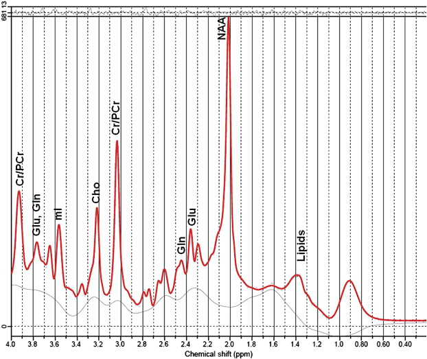
An example of human brain spectrum from parietal gray matter is shown in Figure 5.1.1 . For instance the methyl protons of N -acetyl-aspartate (NAA) resonate at 2.01 ppm and free water protons at 4.7 ppm.
5.1.1.2.2
Spin–Spin Coupling
Many biological molecules contain several protons. Because protons possess a small magnetic moment (spin) themselves, they influence each other, thus they affect the magnetic field experienced by nearby protons; this effect is known as spin–spin coupling . a
a Heteronuclear coupling also exists, e.g., between 1 H and 13 C.
In the liquid state this spin–spin interaction is typically canceled through space interaction due to rapid molecular tumbling. In chemical bonds, instead, spin–spin interaction through electrons does not average to zero and is responsible for the “splitting” of resonance lines. This coupling is expressed in units of Hz as it is independent of the externally applied B 0 and only varies with the number (and type) of bonds between the protons.
Each proton will be affected by the spin state of nonmagnetically equivalent protons b
b Magnetically equivalent nuclei have the same chemical shifts (chemically equivalent), plus they have same coupling constants with all other coupled nuclei. For instance, CH 3 protons are magnetically equivalent; therefore, if uncoupled they will appear as a singlet. They have a different chemical environment from CH protons, thus they have a different chemical shift.
in the same molecule. Due to the different chemical shifts and coupling constants, each molecule will display one or a number of peaks (or “resonances”) on the MRS frequency axis, its MRS “signature”.For instance, any proton that is not coupled to another proton would show a “singlet” resonance, i.e., a single peak in the MRS spectrum. This is not the case for coupled spins, for example in lactate, a group of magnetically equivalent protons (CH 3 ) is coupled to the CH proton. The proton in CH can be in one of two states, parallel and antiparallel to B 0 , each affecting the CH 3 protons slightly differently. The CH 3 singlet therefore experiences a “splitting” and appears in a spectrum as a “doublet” of peaks, each with half of the area it would have had if there had been no coupling. The CH proton resonance is in turn coupled to the three protons of CH 3 and affected by their individual spin states, which means that the CH spectrum will therefore show four lines (quartet) with intensity ratios 1:3:3:1 (corresponding to one configuration for all spins up, three possible configurations for two up one down, three configurations for two down one up, and one configuration for all down). For a CH proton coupled to a CH 2 group, we would see instead a “doublet of doublets” that would form a “triplet” of peaks with ratios (1:2:1).
Spin–spin couplings and the multiplets they produce in relation to the underlying molecular structure are thus extremely useful, together with chemical shift information, to identify and assign resonances.
High resolution spectra allowing split resonances to be fully resolved can often be obtained on ex vivo tissue extracts or homogenized solutions at high magnetic field (7 T–14 T).
In vivo MRS spectra have limited resolution and in many cases the line splitting cannot be directly observed. In any case, knowledge of the theoretical splitting allows better modeling of the observed signal.
5.1.1.2.3
Aim of MRS Spectral Analysis
Once an MRS spectrum is collected the aim of the MRS spectroscopist is to correctly identify the resonances in the spectrum and assign them to the corresponding molecules. The greater the concentration of a particular molecule in the VOI, the greater the amplitude of its corresponding MRS signature (resonances). By measuring peak amplitudes, after correct assignment it is possible to calculate the absolute or relative concentration of the molecules from which these peaks originate.
This procedure can give direct and detailed information on the biochemistry within the VOI in a wholly noninvasive fashion. Whilst single-point MRS gives a snapshot view of metabolite concentrations at a specific moment in time, repeated measurements can also be carried out to provide, for instance, dynamic metabolic information.
5.1.1.2.4
Features of MRS Spectra
The main complication in the spectral analysis is that the MRS signatures of many molecules do partially overlap, and this causes an uncertainty associated with each frequency (as explained following), which makes the assignment procedure potentially equivocal.
One of the characteristics of each resonance peak, in fact, is its linewidth (often calculated as the full width at half maximum, FWHM) that depends on its T 2 ∗ (apparent transverse relaxation time constant), related to the compounded effect of local and macroscopic magnetic field inhomogeneities. While the effects of inhomogeneities that are stationary in time can be reversed or accounted for with appropriate acquisition techniques, local magnetic field fluctuations are randomly variable in time and are inherent to the system under study.
As in MRI, MRS data quality can also be characterized by a signal-to-noise ratio (SNR) value, expressing the ratio between resonance peaks arising from a chosen compound and random noise occurring equally at all spectral frequencies.
In addition to random noise, the analysis will be complicated by signals arising from molecules and compounds that are not expected or taken into account explicitly (often this is the case for extremely broad resonances from macromolecules resulting in nonflat spectral baselines).
The ability to discriminate resonances will increase as peak linewidths are minimized and SNR maximized. Linewidths can be improved by optimizing the uniformity of the local magnetic field over the VOI (shimming) prior to the acquisition of MRS data (see Section 5.1.2.2 ). SNR will depend on the acquisition parameters: choice of echo time (TE) and repetition time (TR), acquisition bandwidth (BW), as well as the volume of the VOI (VOI volume ) and the number of spectral averages ( N avg ) collected.
Similarly to MRI, for a singlet resonance peak this can be generally expressed as:
SNR ∼ N avg BW · VOI volume · e − TE T 2 · ( 1 − e − T R T 1 )
In other words, SNR increases linearly with VOI volume , but only with the square root of N avg . Knowledge of T 1 of the substance of interest can allow optimization of SNR per unit time, though in some instances long TRs are preferable to provide insensitivity to pathological T 1 changes. Reduced TE also allows better SNR, however the contribution to the spectra of short-TE macromolecules results in rolling spectral baselines and complicates quantification. Lower readout bandwidths give an SNR advantage, however, the BW cannot be arbitrarily chosen and needs to be large enough to span across the frequencies of resonances from all detectable metabolites.
5.1.1.2.5
Basics of Localized MRS Data Acquisition
The first MRS spectra ever acquired were collected as a rapidly decaying signal or free induction decay (FID). This was measured immediately following a nonspatially selective excitation of a sample in an external (uniform and stationary) B 0 magnetic field. The excitation consisted of a magnetic field ( B 1 ) perpendicular to the B 0 direction and oscillating or rotating at the Larmor frequency corresponding to it. It is therefore common to refer to this magnetic field as a radiofrequency (RF) pulse. In this experiment the FID, contains information from the whole sample experiencing the applied magnetic field B 1 .
However, often it is necessary to define the volume from which the signal originates. The simplest way to achieve a spatial localization of the collected signal is by making sure that the excitation pulse is “on resonance” only for a selected VOI as follows.
The B 1 pulse can be designed to excite only a narrow slab of a sample exactly as in MRI by applying at the same time a magnetic field that has the same direction of B 0 but varies in space, i.e., a magnetic field gradient. Employing three subsequent B 1 pulses with gradients along three orthogonal directions defines a 3D VOI where the three slabs overlap. One of the most commonly employed sequences is equivalent to a double-echo spin-echo and employs B 1 pulse with typical flip angles of 90°, 180°, 180° and was originally suggested in 1984 with the acronym of PRESS (point resolved spectroscopy). If the three B 1 pulses are all producing 90° flip angles another extremely common MRS sequence is produced, commonly referred to with the acronym of STEAM (stimulated echo acquisition mode ), where it is only the resulting stimulated echo that contains the localized spectral information desired. (Note: See Section 5.1.3.5 for a discussion of the relative merits of these two sequences in relation to spinal cord MRS.)
Signal from multiple VOIs from a slab or volume of tissues can also be collected; the technique is called chemical shift imaging (CSI) or MR spectroscopic imaging (MRSI). For instance, in PRESS-based CSI, the three overlapping slabs define a large VOI that is further subdivided into smaller elements by means of phase encoding as in conventional MRI. c
c This “phase encoding” is applied along one, two, or three orthogonal directions for 1D-CSI, 2D-CSI, and 3D-CSI, respectively.
5.1.2
1 H MRS in the Spinal Cord
5.1.2.1
Introduction
Twenty years passed after the first human in vivo MRS experiment, before localized MRS in the spinal cord was performed. The group that first investigated it was based in the Institute of Neurology in University College London in 1997–2000. It took a further four years for other groups to pick up the challenge. Currently there are still only a few groups worldwide that routinely undertake spinal cord MRS, and one of the reasons for this is that it is technically challenging.
A selection of studies that have reported spinal cord MRS methodology are listed in Table 5.1.1 and will be referred to in more detail in the next sections.
| Publication | Year | B 0 | RF Coil | Sequence | Water Supp. | Cardiac Trigger | TR (s) | TE (ms) | NSA | Voxel Size | Position | Shim Method | Subject Group |
|---|---|---|---|---|---|---|---|---|---|---|---|---|---|
| Gomez-Anson | 2000 | 1.5 T | Volume | PRESS | CHESS | – | 3 | 30/144 | 256 | 9 × 60 × 40 | – | – | Healthy |
| Cooke | 2004 | 2 T | Surface | PRESS | CHESS | Yes (400 ms) | 3 | 30 | 256 | 9 × 7 × 35 | Above C2 | B 0 mapping | Healthy |
| Kendi | 2004 | 1.5 T | Phased array | PRESS | MOIST | – | 1.5 | 35 | 196 | 6 × 6 × 50 | C3–C7 | Auto | MS |
| Kim | 2004 | 1.5 T | Flexible surface | STEAM | CHESS | – | 2 | 30 | 256 | – | Spinal tumor mass | – | Spinal mass lesions |
| Blamire | 2007 | 2 T | Surface | PRESS | CHESS | Yes (400 ms) | 3 | 30 | 256 | 9 × 7 × 35 | Center C3 | B 0 mapping | MS |
| Ciccarelli | 2007 | 1.5 T | Saddle | PRESS | CHESS | Yes (150 ms) | 3RR | 30 | 192 | 6 × 8 × 50 | C1–C3 | Manual | MS |
| Edden | 2007 | 3 T | Flexible surface | 1D-PRESS CSI | Dual HS pulses | No | 2200 | 144 | 64 | FOV 10 × 12 × 90 | Medulla-C3 | FASTMAP | Healthy |
| Henning | 2008 | 3 T | 12 Channel spine | PRESS | CHESS | Yes (300 ms) | 2 | 42 | 512 | 6.5 × 8.5 × 27 | C2–C3,Thoracic lumbar | B 0 mapping | Healthy + Various pathologies |
| Holly | 2009 | 1.5 T | – | PRESS | – | Yes | 1.5/3 | 30 | 256 | 10 × 10 × 20 | Center C2 | Manual | Cervical Spondilotic myelopathy |
| Ciccarelli | 2010 | 1.5 T | Saddle | PRESS | CHESS | Yes (150 ms) | 3RR | 30 | 192 | 6 × 8 × 50 | C1–C3 | Manual | MS |
| Marliani | 2010 | 3 T | 8 Channel spinal | PRESS | CHESS | – | 2 | 35 | 396 | 7 × 9 × 35 | C2–C3 | Auto non- triggered | MS |
| Carew 6 | 2011 | 3 T | Volume | PRESS | CHESS | – | 2 | 35 | 256 | 8 × 5 × 35 | Above C2 | B 0 mapping | ALS at risk |
| Kachramanoglou | 2011 | 3 T | 8 Channel | PRESS | CHESS | – | 3 | 30 | ∼160 | – | C1–C3 | B 0 mapping | MS and brachial plexus |
| Elliott | 2011 | 3 T | – | PRESS | – | – | 3 | 30 | ∼220 | 10 × 10 × 20 | C1–C3 | Auto | Whiplash |
| Hock | 2011 | 3 T | 16 Channel | PRESS | VAPOR/None | Yes | >2.5 | 30 | 512 | 6 × 9 × 35 | – | FASTERMAP | Healthy |
Related posts:

Stay updated, free articles. Join our Telegram channel

Full access? Get Clinical Tree


