Fig. 1
Overview of the components involved for the 3D reconstruction of the spine from radiographic images
This chapter presents the different techniques involved for generating the 3D reconstruction of a patient’s spine using biplanar radiographs. The personalized 3D reconstruction of the spine enables both the visualization from calibrated biplanar radiographic images and the clinical assessment of spinal deformities in a wide range of pathologies. The remainder of this chapter is structured as follows. Section 2 presents an overview of the evolution of 3D reconstruction systems. In Sect. 3, the approaches for calibrating the X-ray scene are described, while Sect. 4 focusses on the 3D modelling of the spine using either point-based or feature-based representations. For the selected applications, results are given in Sect. 5. Finally, we conclude this chapter in Sect. 6.
2 Evolution of 3D Reconstruction Systems
2.1 First Generation
For years, research in the field of biomechanics has focused tremendously on the analysis of spinal deformities in 3D. The elaboration of complex biomechanical models required rigorous clinical experimentations, as well as quantitative evaluations of the patient’s posture and movement analysis in three dimensions. In 1971, Panjabi and White illustrated the importance of studying the spine in three dimensions (3D), with 6 degrees of freedom. A number of techniques for 3D measurements, imaging and modelling of the spine were developed [1, 9, 11, 24, 34]. Since 1992, an imaging system installed at the Sainte-Justine Hospital Research Center enabled to perform the 3D reconstruction of bony structures from radiographic images (Fig. 2). The proposed system was based on the calibration principle of the Direct Linear Transform (DLT), which implicitly includes the geometric parameters in the coefficients of the projection matrices obtained linearly by an inversion of the matrix. Using a Plexiglass cage with encrusted steel pellets, the 2D/3D configuration could be determined in a linear fashion. This tool was used in over 6,000 patient visits for research purposes, in addition to other applications such as surgical simulations and biomechanical analysis of the spine. The system was also used to improve the quality of diagnosis and follow-up exams for patients with idiopathic scoliosis. Finally, this 3D imaging system was used in a number of other projects involving computer assisted surgery and personalization of models.
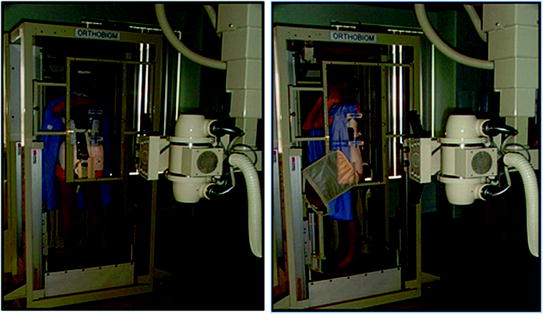

Fig. 2
One of the first 3D reconstruction systems installed at the Sainte-Justine Hospital in 1992, where a plexiglass cage with embedded pellets is used to calibrate the X-ray scene. The patient is turned from the frontal to sagittal position to obtain biplanar radiographs
In order to facilitate the 3D reconstruction of scoliotic trunks, algorithms based on the explicit modelling of calibration matrices were used to calibrate the X-ray scene [7, 8]. However, this particular system required for the patient to be placed in a fixed positioning system while wearing a calibration vest during the radiographic acquisition (Fig. 3), necessitating calibrated images in order to obtain the 3D reconstruction of the spine. Because of the inherent limitations of the system used for research purposes, it became clear such a device could not be deployed in other clinics and thereby exploiting the benefits of 3D reconstruction of the spine. This ultimately limits the universal access to such a technology in a routine setting to assess spinal deformations in 3D.
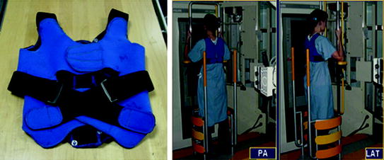

Fig. 3
Left Calibration vest worn by the patient and the positioning system used at the Sainte-Justine Hospital. The calibration vest has embedded radio-opaque markers visible on the biplanar to self-calibration the scene using fiducial points closer to the patient’s skin. Right Positioning system to minimize patient motion between biplanar acquisitions
2.2 New Generation of 3D Reconstruction Systems
The ionization dose given to the patient using conventional radiography in not negligible, and can ultimately induce a risk of cancer or leukaemia with repetitive acquisitions [53], in addition to offer images of average quality. A low-dose imaging system based on the invention of Georges Charpak (1992 Nobel prize of physics [5]) was developed by EOS imaging (Paris, France) to generate high-quality radiographic images, while considerably reducing ionization doses. A first evaluation of the prototype was conducted at the St-Vincent de Paul Hospital in Paris in 1995. Improvements to the system were introduced in order to increase the resolution and reduce the image acquisition time due in part to the new technologies in radio-sensitive detectors. The EOS system (Fig. 4) can acquire simultaneously biplanar radiographic images and includes a software (sterEOS) to perform the reconstruction of bony structures. This system is now installed in over 30 countries, including the US, Canada and Germany.
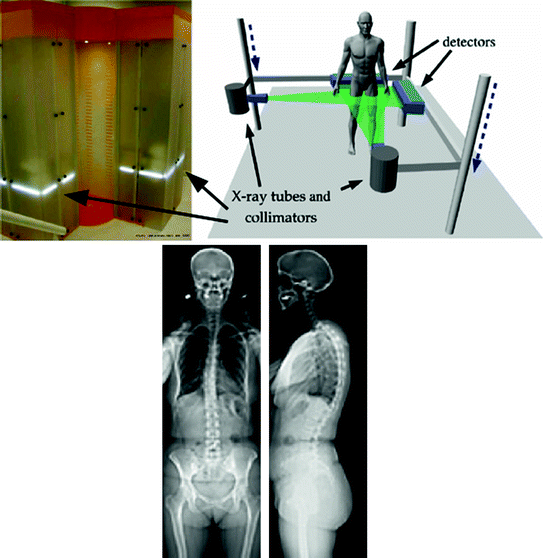

Fig. 4
EOS system (EOS imaging ©) enabling the head-to-toe reconstruction of bony structures (adapted from [13])
3 Radiographic Calibration
In order to generate three-dimensional models from stereo-radiographic images, the radiographic scene must first be calibrated so to calculate a 3D coordinate for a set of 2D projection coordinates. This section presents the various approaches that can be used to perform the calibration process.
3.1 Linear Calibration Techniques
The first 3D reconstruction techniques were based on stereo-radiography, such as the Direct Linear Transform (DLT), which have been widely used for this application [2, 10, 12, 44]. These methods require the use of a large calibration object with fiducial markers of known 3D coordinates and their projection on the 2D images to estimate the intrinsic parameters of the radiographic configuration. However, this setup makes the reconstruction algorithm vulnerable to patient motion between the exposures by creating inconsistencies in the calibration and patient stereo geometries, in addition to being cumbersome in a routine clinical setup. To overcome these limitations, Cheriet et al. [8] proposed an explicit calibration procedure to estimate the X-ray source and film geometric configuration relative to the patient’s frame of reference from the content of the images (using a non-rigid calibration vest). The general idea was to adjust the geometric parameters that describe the radiographic setup in such a way as to minimize landmark retro-projection errors. The algorithm used matched calibration landmarks identified on a pair of X-rays and approximate geometric parameters to calibrate the images, while still requiring a calibration object to iteratively update the radiographic system’s parameters until it converges to a stable state which reflects a valid solution. These approaches are not suitable for the new generation EOS systems (Sect. 2.2).
3.2 Non-linear Calibration Techniques
Methods have been proposed to enable the 3D reconstruction of the spine from biplanar X-ray images without requiring a bulky object or calibration vest, thus introducing the 3D evaluation of spinal deformities in a wide range of clinical setups [28]. Still, they require an expert to manually identify and match landmarks on the anatomy to calibrate and subsequently reconstruct a model in 3D. In fact, to generate a 3D model of the patient’s spine from biplanar radiographs, certain points (anatomical landmarks) on the vertebrae within the image have to be located in order to obtain a 3D model of the scoliotic spine using a triangulation algorithm [12]. Typically, this identification is performed manually by an expert operator and consists of locating anatomical landmarks on a coronal and sagittal radiograph (Fig. 5). However, it is difficult to accurately identify low-level primitives such as exact points and to match them accurately on a pair of views. Thus the repeatability of this procedure cannot be assured. Furthermore this task is time-consuming, tedious and error-prone, and the quality of the 3D reconstruction is directly linked with the precision of 2D localization. Panjabi discussed in detail errors that arise when manually identifying anatomical landmarks [48].
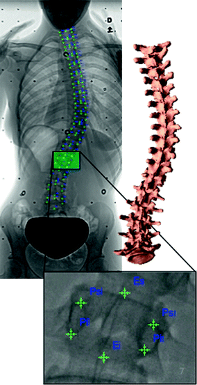

Fig. 5
Manual anatomical landmark identification on the X-ray for the personalized 3D reconstruction of the scoliotic spine. Visible markers are the identified landmarks on each vertebra which are used in the self-calibration of an X-ray scene
Due to these pitfalls, clinical 3D assessment of the deformity during a patient’s visit is therefore not possible. Moreover, because current self-calibration techniques rely on single point correspondences between the biplanar images which offer sparse data with low redundancy [7, 47], this generates multiple local minimums when optimizing the non-linear equation system describing the radiographic setup. Local correspondences also rely on the assumption that a point on an object’s surface appears the same in the biplanar images in which it is visible. However due to the phenomena exhibited by the X-ray modality, punctual point matches are not necessarily a reliable matching feature for 3D bone reconstruction. For these reasons, region-based comparisons via surface integration [65] may not only improve the quality of 3D calibration results by incorporating additional data such as high-level corresponding geometrical primitives (curves, surfaces), but can reduce the number of degrees of freedom to solve the equation system.
Furthermore, the self-calibration of a biplanar X-ray system is a complex mathematical problem difficult to solve. In order to improve the quality of current self-calibration techniques [7, 28] which rely on iterative algorithms optimizing the retro-projection of sparse data points to solve a complex system of non-linear equations, it is necessary to incorporate additional data into the system and to incorporate additional mathematical constraints (e.g. Kruppa’s equations and epipolar geometry [21] which are mathematical constructs frequently used for camera self-calibration from a sequence of images). Additional constraints allow the reduction of the number of degrees of freedom in the system of equations without additional data. Using corresponding high-order geometrical primitives (line segments, ellipses, curves, etc.) instead of only point correspondences for the resolution of the self-calibration problem can drastically increase the quantity of data fed into the algorithm. Geometric parameters such as the rotation and translation components of the camera configuration can be determined based on shape information taken from the biplanar projection views, such as with mathematical high level geometrical primitives (lines or ellipses) [52] or with intrinsic properties such as tangent vectors and maximal curvature points to [16]. Although these properties have yet to be used for orthopaedic imaging, properties such as geometrical torsion which describes the 3D phenomena in AIS [51] can be used in the context of calibrating an X-ray scene to establish the 2D-3D relationships for tangential and curvature characteristics extracted from 3D spinal curves [40]. Thus by determining the 3D parameters of a Frenet-Serret frame for example, based on the 2D information collected from the projection images, this set of information can be exploited in a 2D-3D correspondence framework.
3.3 Image-Based Self-calibration
Progressing towards an automated calibration technique therefore involves segmenting anatomical shapes or high level geometrical primitives which can be accurately matched on the X-ray images. Segmentation of bony anatomical structures remains however a challenging problem due to overlapping organs in the thoracic region and low image signal-to-noise ratio. Automatic spine segmentation approaches have been sparsely explored by using machine learning approaches based on localized texture parameters, morphological descriptions in dynamic programming [19] or from Active Shape Models (ASM) using templates from learning data [57]. Based on the work of Cheng et al. [6] which presented a Bayesian approach that uses manually labelled data for parcellation applications, spatial relationships can be used, where the segmentation of the spine shape relied mostly on prior anatomical knowledge information taken from an atlas prior [32]. The core idea of using a manual training set for incorporation of prior statistics and class conditional densities can be transposed in such a work to model the variation distribution of vertebral boundaries by constraining image intensities. This approach is motivated from the fact that segmenting spine contour silhouettes from the biplanar images would offer high level geometrical primitives which could be used to establish 2D-3D correspondence metrics in the self-calibration optimization scheme. Hence, visual reconstructions can be exploited as high-level anatomical primitives, which are subsequently matched between the biplanar X-rays to determine the 2D-3D relationship of the radiographic scene by self-calibration [27]. Hence, two distinct correspondence features were developed for the discrete non-linear optimization procedure and are described below.
3.3.1 Visual Hull Reconstruction
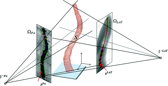
This section exposes an approach which has been extensively investigated in visual robotics, by adapting an algorithm derived from the shape-from-silhouette principle for a visual hull reconstruction of medical images. First, the spine shapes are first segmented on the images using a prior knowledge Bayesian framework [32] to capture vertebral contour, width, and rotation information in the frontal and sagittal planes. This facilitates the partitioning problem for complex pathological deformations. The silhouettes of the segmented anterior portion of the spine on the biplanar images are then used for the visual hull reconstruction of the global shape of the spine as illustrated in Fig. 6. A visual hull depends both on the spine silhouettes  with
with  and on the camera viewing parameters
  such as
  which remain to be determined. Once the silhouettes are obtained from the images [32], the reconstruction is based on the concept of visual hulls. Formally, the visual hull of the 3D spine S with respect to the viewing plane
  , denoted by
  , is a volume in space such that for each point P in
  and each camera viewpoint
  in
in  , the half-line from
  through P contains at least one point of S [39]. This definition states that the visual hull consists of all points in space whose images lie within all silhouettes viewed from the viewing region. Hence, the visual hull is the maximal object that has the same silhouettes as the original object, as viewed from the viewing region. The segmented object and spine silhouettes are projected into the 3D space by conical visual hulls in the projective projection model, and its projection should coincide with its silhouette on
  such that
  . By computing the intersection of the visual hulls projected from both images (i.e. biplanar viewing directions), the estimation for the shape of the spine is obtained according to the current projection parameters
  .
.
 with
with  and on the camera viewing parameters
  such as
  which remain to be determined. Once the silhouettes are obtained from the images [32], the reconstruction is based on the concept of visual hulls. Formally, the visual hull of the 3D spine S with respect to the viewing plane
  , denoted by
  , is a volume in space such that for each point P in
  and each camera viewpoint
  in
in  , the half-line from
  through P contains at least one point of S [39]. This definition states that the visual hull consists of all points in space whose images lie within all silhouettes viewed from the viewing region. Hence, the visual hull is the maximal object that has the same silhouettes as the original object, as viewed from the viewing region. The segmented object and spine silhouettes are projected into the 3D space by conical visual hulls in the projective projection model, and its projection should coincide with its silhouette on
  such that
  . By computing the intersection of the visual hulls projected from both images (i.e. biplanar viewing directions), the estimation for the shape of the spine is obtained according to the current projection parameters
  .
.
Fig. 6
Principal of the visual hull 3D reconstruction of the global spine shape based on the projected silhouette  and
and  on the biplanar radiographic views. The shape of the object S is estimated by the intersection of both visual cones issued from viewpoints V, offering a sparse and approximate representation of the global spine shape
 and
and  on the biplanar radiographic views. The shape of the object S is estimated by the intersection of both visual cones issued from viewpoints V, offering a sparse and approximate representation of the global spine shape
3.3.2 Geometric Torsion of the Scoliotic Spine
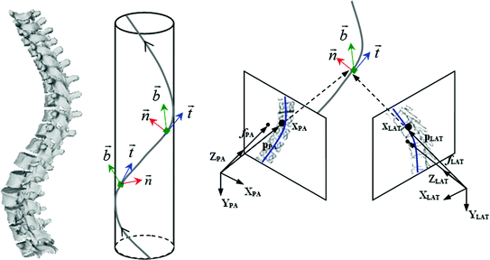
Due to the 3D nature of idiopathic scoliosis, the natural curvature properties of the spinal curve can also exploited in the refined optimization of the radiographic parameters, by using the geometrical torsion of the spine measuring the amount of deviation (divergence) of the curved line from the plane determined by the tangent t and normal n vectors [51]. In scoliosis, geometric torsion is related to the amount of helicoidal deformity in the spine. It can be defined as a local geometric property of the 3D curved line passing through thoracic and lumbar vertebrae that measures the amount of helicoidal deviation of the vertebrae, without specific relation to the rotation and deformation of the vertebrae themselves. The continuous parametric 3D B-spline spinal curve  that passes through the center of the spine was represented by Frenet’s formulas in order to calculate the geometric torsion as portrayed in Fig. 7. Ultimately, 2D-3D correspondences and a derived relationship which uses Frenet frames to extract 2D information from the image curves are used, and compute their 3D measurements. First, let
  be a regular curve parameterized by arc length in
  . If the Frenet (tangent, normal, binormal) frame F = {T, N, B} and the curvature are known at
  , a local approximation is obtained as follows:

 that passes through the center of the spine was represented by Frenet’s formulas in order to calculate the geometric torsion as portrayed in Fig. 7. Ultimately, 2D-3D correspondences and a derived relationship which uses Frenet frames to extract 2D information from the image curves are used, and compute their 3D measurements. First, let
  be a regular curve parameterized by arc length in
  . If the Frenet (tangent, normal, binormal) frame F = {T, N, B} and the curvature are known at
  , a local approximation is obtained as follows:
Fig. 7
The scoliotic spine represented as a helical line which can be uniquely determined by its geometric torsional quantity. The concept of geometric torsion ( ) is illustrated by the moving trihedron formed by the tangential t, normal n, and binormal b vectors
 ) is illustrated by the moving trihedron formed by the tangential t, normal n, and binormal b vectors
(1)
Hence,  and
and  are defined as the curves representing the spine centerline derived from the segmented silhouettes
  on the PA and LAT images respectively. Therefore for each value of u such that
 ![$$u = [0,2{\uptau },3{\uptau }, \ldots ,1]$$](/wp-content/uploads/2016/12/A312884_1_En_6_Chapter_IEq21.gif) and
and  is the equidistant step-size, a node in the tangent space
  is defined, where
  and
and  are the image projection coordinates of X,
  the orientation of projected tangent in the image planes, and
  the image curvatures, with i representing the biplanar X-rays. Here, the 3D position X and tangent T are computed using standard methods [22]. To determine the normal N and the 3D curvature
  at a 3D space curve point on
  from biplanar views, the mathematical relationship proposed by Li and Zucker [40] can be used where the 3D normal N, the curvature
  and the parameters from the viewing geometry is formulated as:

where  , p is determined from the vector pointing to the projection in the image plane and f is the vector pointing to the image center, both in the camera coordinate system. The
  parameter is the depth computed from calibration while t is the local tangent vector on the 2D image. The curvature can then be computed as
  , given the constraint
  . Hence, the normal vector can be determined by
  .
.
 and
and  are defined as the curves representing the spine centerline derived from the segmented silhouettes
  on the PA and LAT images respectively. Therefore for each value of u such that
 ![$$u = [0,2{\uptau },3{\uptau }, \ldots ,1]$$](/wp-content/uploads/2016/12/A312884_1_En_6_Chapter_IEq21.gif) and
and  is the equidistant step-size, a node in the tangent space
  is defined, where
  and
and  are the image projection coordinates of X,
  the orientation of projected tangent in the image planes, and
  the image curvatures, with i representing the biplanar X-rays. Here, the 3D position X and tangent T are computed using standard methods [22]. To determine the normal N and the 3D curvature
  at a 3D space curve point on
  from biplanar views, the mathematical relationship proposed by Li and Zucker [40] can be used where the 3D normal N, the curvature
  and the parameters from the viewing geometry is formulated as:
(2)
 , p is determined from the vector pointing to the projection in the image plane and f is the vector pointing to the image center, both in the camera coordinate system. The
  parameter is the depth computed from calibration while t is the local tangent vector on the 2D image. The curvature can then be computed as
  , given the constraint
  . Hence, the normal vector can be determined by
  .
.3.3.3 Self-calibration by Means of Optimization of the Radiographic Parameters
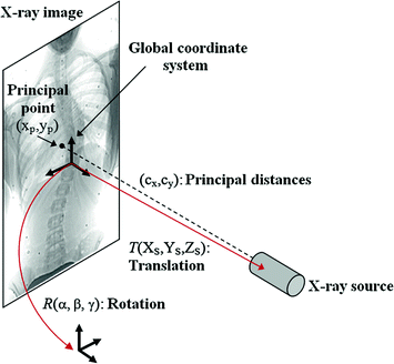
The proposed self-calibration algorithm involves explicit use of the description of the calibration matrices  in order to estimate the geometrical parameters of the radiographic setup leading to an optimal 3D reconstruction of all the spine’s vertebrae [7, 8]. The projective matrices
  used for the stereo-reconstruction of 3D landmarks are modeled as:

where  is the rotation matrix defined by angular
  ,
,  is the translation vector
  . Intrinsic parameters are modeled by the
  ,
,  coordinates of the principal point and
  ,
,  as the principal distances. These parameters are described schematically in Fig. 8. A rough estimation of these parameters is extrapolated from a small object of known dimensions taken in the radiographic scene [28]. Hence the geometrical parameters
  ,
,  are subsequently updated based on an iterative nonlinear optimization process with regards to the global shape of the spine, following the objective function:

 in order to estimate the geometrical parameters of the radiographic setup leading to an optimal 3D reconstruction of all the spine’s vertebrae [7, 8]. The projective matrices
  used for the stereo-reconstruction of 3D landmarks are modeled as:
(3)
 is the rotation matrix defined by angular
  ,
,  is the translation vector
  . Intrinsic parameters are modeled by the
  ,
,  coordinates of the principal point and
  ,
,  as the principal distances. These parameters are described schematically in Fig. 8. A rough estimation of these parameters is extrapolated from a small object of known dimensions taken in the radiographic scene [28]. Hence the geometrical parameters
  ,
,  are subsequently updated based on an iterative nonlinear optimization process with regards to the global shape of the spine, following the objective function:
(4)

Fig. 8
Illustration of the ten geometric parameters described within the context of the X-rays
This cost function combines two image-based criterions. The first component maximizes the intersected region between the segmented silhouette and the projection of the shape of the spine computed by the visual hull 3D reconstruction, and minimizes isolated regions such that:

where  is the segmented silhouette on image plane i,
  is the projection of the global visual hull shape S, and
  the image plane domain defined in the
  space. The second component evaluates the difference between the back-projection of the equidistant 3D Frenet frames taken at
  intervals along the 3D spinal curve
  and the 2D curves
  of the X-ray images:
![$$\begin{aligned} E_{\text{torsion}} (\xi_{i} ) = \sum\limits_{j = 0}^{N} & [{\parallel }x_{{\alpha_{i} (j/N)}} - {\varPi }^{i} ({\mathbf{X}}_{{C_{k} (j/N)}} ){\parallel }^{2} \\ & \, + {\parallel }t_{{\alpha_{i} (j/N)}} - \varPi^{i} ({\mathbf{T}}_{{C_{k} (j/N)}} ){\parallel }^{2} \\ & \, + {\parallel }\kappa_{{\alpha_{i} (j/N)}} - \varPi^{i} ({\mathbf{K}}_{{C_{k} (j/N)}} ){\parallel }^{2} ] \end{aligned}$$](/wp-content/uploads/2016/12/A312884_1_En_6_Chapter_Equ6.gif)
where N is the number of Frenet frames along the spinal curve. The first two terms evaluate the Euclidean distance between the analytical projection of X and T from standard perspective transformation formulae using the current estimate of the geometrical parameters and the image measures x and t respectively. The third term measures the difference in curvature values  using (14). The method uses a bundle adjustment approach based on an iterative nonlinear optimization process. The Levenberg-Marquardt algorithm is used for optimization, iterating until the correction to the geometric parameters becomes negligible [8]. The set of parameters and projection matrices is therefore regenerated and this procedure is repeated until the system reaches a steady state, where the distance between the observed and computed projection falls to a minimum. To avoid local minima, a directional optimization approach is used to obtain a first, coarse solution which is accurate enough to be used as an initial guess. Moreover, higher reliability of the torsion parameters is ensured in the optimization scheme by enforcing regularity in the Tikhonov sense with the term
  . This helps to compensate the instability of the curvature parameters for patients with strong deformations which can affect the convergence of the algorithm. The regularization term acts as a dampening factor, controlling the quality of these parameters by penalizing terms exhibiting very high tangential and torsional values.

(5)
 is the segmented silhouette on image plane i,
  is the projection of the global visual hull shape S, and
  the image plane domain defined in the
  space. The second component evaluates the difference between the back-projection of the equidistant 3D Frenet frames taken at
  intervals along the 3D spinal curve
  and the 2D curves
  of the X-ray images:
![$$\begin{aligned} E_{\text{torsion}} (\xi_{i} ) = \sum\limits_{j = 0}^{N} & [{\parallel }x_{{\alpha_{i} (j/N)}} - {\varPi }^{i} ({\mathbf{X}}_{{C_{k} (j/N)}} ){\parallel }^{2} \\ & \, + {\parallel }t_{{\alpha_{i} (j/N)}} - \varPi^{i} ({\mathbf{T}}_{{C_{k} (j/N)}} ){\parallel }^{2} \\ & \, + {\parallel }\kappa_{{\alpha_{i} (j/N)}} - \varPi^{i} ({\mathbf{K}}_{{C_{k} (j/N)}} ){\parallel }^{2} ] \end{aligned}$$](/wp-content/uploads/2016/12/A312884_1_En_6_Chapter_Equ6.gif)
(6)
 using (14). The method uses a bundle adjustment approach based on an iterative nonlinear optimization process. The Levenberg-Marquardt algorithm is used for optimization, iterating until the correction to the geometric parameters becomes negligible [8]. The set of parameters and projection matrices is therefore regenerated and this procedure is repeated until the system reaches a steady state, where the distance between the observed and computed projection falls to a minimum. To avoid local minima, a directional optimization approach is used to obtain a first, coarse solution which is accurate enough to be used as an initial guess. Moreover, higher reliability of the torsion parameters is ensured in the optimization scheme by enforcing regularity in the Tikhonov sense with the term
  . This helps to compensate the instability of the curvature parameters for patients with strong deformations which can affect the convergence of the algorithm. The regularization term acts as a dampening factor, controlling the quality of these parameters by penalizing terms exhibiting very high tangential and torsional values.
4 3D Reconstruction of the Spine
In this section, we present the different methods for generating a 3D model of a vertebra or spine from radiographic images. These methods are categorized in the following classes: point-based, contour-based and statistical methods. We then present a hybrid statistical and image-based approach to generate personalized 3D reconstructions based on geometrical properties in Sect. 4.4.
4.1 Point-Based Methods
The 3D reconstruction of point-based models is usually performed manually by an expert operator and consists of locating six corresponding anatomical landmarks (2 endplate midpoints + 4 pedicle extremities) on each vertebra from T1 (first thoracic vertebra) to L5 (last lumbar vertebra) on a coronal and sagittal X-ray (Fig. 5). Additional non-stereo corresponding point (NSCP) landmarks on the spinous processes or on the corners of the vertebral body may be added to obtain a more refined and detailed geometry of the 3D vertebrae by deforming generic models using an epipolar geometry [45]. However, it is difficult to identify with precision low-level primitives such as exact points and to match them accurately on a pair of views. Thus the repeatability of this procedure can not be assured. As discussed in Sect. 3.2, the manual identification of landmarks is a long and complex process, which cannot ensure repeatability over multiple raters.
4.2 Contour-Based Methods
Local correspondence also relies on the assumption that a point on an object surface appears the same in the biplanar images in which it is visible. However due to the intrinsic properties exhibited by the X-ray modality, local correspondence is not necessarily a reliable feature for 3D bone reconstruction. Non-stereo corresponding contours (NSCC) methods have been proposed for the 3D reconstruction of anatomical objects demonstrating few corresponding features on the biplanar X-rays, such as for long bones (femur) or the pelvis [38]. The approach optimizes 3D deformations of prior models by minimizing the object’s projection from manually identified 2D contours. These techniques demonstrated promising results but are still limited to the manual identification of curves along the edges of long bony structures. For these reasons, variational methods with a region-based component have been applied to multi-view stereo reconstruction as an alternative to local correspondence [65]. Unlike local correspondence, there is no matching of points between pairs of images for consistency, but instead the comparison is integrated over regions. This can not only improve the precision of reconstruction results by incorporating additional data such as high-level corresponding geometrical primitives (curves, surfaces), but reduces manual intervention required to identify specific anatomical landmarks on the X-rays.
4.3 Statistical Methods
In order to reduce inaccuracies on the 2D localization of landmarks and to be a clinically useful procedure, previous studies were conducted to propose more automated methods. Initial attempts were based on vertebral template matching [46, 56], and feature-based by using active shape models (ASM) [57] or Hough transforms [23, 64], to detect dominant characteristics (corners, edges) from the vertebral shape body. Still, these techniques were ineffective towards noise and varying appearance in shape. Statistical shape models, and more recently 2D-3D registration methods, have been the focus of increased attention for the 3D reconstruction of the human spine. A variety of methods have been proposed in the previous years for image to physical space (patient) registration. While some have used preoperative 3D models from CT or MR images to register with 2D X-ray or fluoroscopic images from gradient amplitudes [20, 41, 60], Fleute and Lavallee have used statistical a priori knowledge of the 3D geometric shapes in order to model the 2D vertebral shapes by applying point distribution models (PDM) [17]. Similar approaches introduced by Lorenz et al. [43] and Vrtovec et al. [63] have used PDM methods from training statistical shape models, thus automatically capturing the geometrical knowledge of the principal modes of variation to isolate 3D vertebrae from tomography images. A method proposed to use a priori knowledge of the vertebral shape using eight morphologic descriptors of the vertebral body to accurately estimate the geometrical model [50]. The obtained model would be manually refined by projecting the spine’s silhouette on the X-rays. Inference-based optimization refinements were subsequently presented to obtain an accurate estimate of the vertebra’s orientation and 3D locations [14]. Still, these approaches remain highly supervised by an operator to manually identify landmarks. Benameur et al. [3] proposed a 3D-2D registration method for vertebrae of the scoliotic spine. In this case, the geometric knowledge of isolated normal vertebrae is captured by a statistical deformable template integrating a set of admissible deformations, and expressed by the first modes of variation in a Karhunen-Loeve expansion. However, none of these methods have attempted to integrate a statistical model taking into account the set of admissible deformations for the whole scoliotic spine shape. Another drawback from most methods is that each vertebra is treated individually instead of as a whole articulated model which may include the global 3D deformation of the spine. Hence in order to account for the global geometrical representation of scoliotic deformities, a variability model (mean and dispersion) of the whole spine allowed increasing the accuracy of the 2D-3D registration algorithm by incorporating knowledge-based inter-vertebral constraints [4]. Klinder et al. [35] has transposed these 3D inter-vertebral transformations to accomplish the segmentation of the spinal cord from CT-scan images. In fact, 3D spinal curve analysis where a model of the curvature of the vertebral column describing the relationship between vertebrae has been particularly useful for 3D medical image analysis of the spine. Because of the intricate and tortuous 3D nature of scoliosis, automated curved planar reformation (CPR) techniques have been presented [62] in order to increase visualization of the deformity by transforming the orthogonal and transverse references to a spinal coordinate system. Furthermore, CPR has been used to assist in the spine segmentation problem using a reformed 3D spinal centerline [33] or by exploiting the approximate proximity of vertebrae along the centerline [18].
Stay updated, free articles. Join our Telegram channel

Full access? Get Clinical Tree


