Statistical Shape Models of the Spine

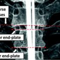
and 3D points $p_{i}^{j}$ . The rigid transformations $T_{i}$ describe the relative position and orientation of each sub-model, and the points $p_{i}^{j}$ describe the local shape in the coordinate system associated with the ith sub-model. An example of anatomical landmarks that can be used to describe the shape of a vertebra is shown in Fig. 1. In this case, only the vertebral end-plates and pedicles are used, which leads to a compact model. However, more landmarks could be used to better describe the shape of the vertebral body or processes. In order to obtain the position and orientation of a vertebra with respect to a global frame of reference, several transformations will need to be composed (see Fig. 2, for instance).

Fig. 1

Example of local anatomical landmarks that can be used to model shape of vertebra. Top lateral view. Bottom anterior view. 1 Center of the superior end plate. 2 Center of the inferior end plate. 3 Top of the right pedicle. 4 Bottom of the right pedicle. 5 Top of the left pedicle. 6 Bottom of the left pedicle

Fig. 2

Relative rigid transformations are used to represent a spine as an articulated object. To obtain absolute positions and orientations with respect to a global frame of reference, one would need to compose a series of inter-vertebral transformations. For instance, the position and orientation of the third vertebra from the bottom would be obtained by applying the rigid transformation $T_{0} \circ T_{1} \circ T_{2}$ to the global frame of reference

This representation of the spine is both intuitive and useful. The spine is a complex anatomical structure, which supports a large portion of our body weight and yet remains flexible enough to allow for complex motions. It includes the vertebrae as well as a variety of soft-tissues (inter-vertebral discs, ligaments, etc.). Vertebrae do not deform significantly in typical circumstances, but because they sit on top of one another; the orientation and position of one vertebra influence its direct neighbors. These relative transformations between neighboring vertebrae would not be captured correctly by a simple set of points and would result in an overestimation of the variability of the spine’s geometry.

2.1 Reconstructing Articulated Models from Existing 3D Data

Articulated representations can be obtained from several sources. Most medical imaging modalities that are routinely applied to the spine can be used to produce articulated spine models. The exact procedure used to extract the articulated models, as well as their accuracy will vary. However, clinical imperatives are likely to decide the imaging modality and posture of the patient.

Volumetric modalities such as computed tomography (CT), magnetic resonance (MR), and even 3D ultrasound can be processed by registering template vertebral models, manually identifying a predefined set of anatomical landmarks, or computing spine-based coordinate systems as part of a curve planar reformation approach [42]. The vast majority of CT or MR scanners require the patient to lie down. Therefore, one has to be very conscious that the variability encoded in the articulated statistical model will represent the anatomical variations for this particular posture.

Traditional bidimensional modalities can also be used to recreate articulated models of the spine. More than one image will generally be necessary to remove the ambiguities that are inherent to 2D images. The most common case in this category is the reconstruction of 3D models of the spine from multiple radiographs (see Chap. 5 of this book for an in-depth discussion). In essence, a human expert provides a computer program with indications about the matching locations in the different radiographs. A three-dimensional model can then be reconstructed by performing triangulation on the matched image coordinates. The way the human expert interacts with the computer program and how the computer program uses these interactions to perform matching varies significantly from one system to another.

Many methods that use an articulated statistical shape model can be used to extract new articulated models with relative ease. For instance, Klinder et al. [25] and Rasoulian et al. [35] used articulated models as part of segmentation methods of the spine applied to CT (computed tomography). The three-dimensional reconstruction of the spine from multiple radiographs was also performed with the help of an articulated statistical shape model [4, 29], and even ultrasound segmentation has been considered for an articulated biomechanical shape prior [20].

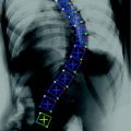
In order to illustrate the different concepts presented in this chapter and demonstrate the use of certain techniques, we will use a database of approximately 300 scoliotic patients that was collected at the Sainte-Justine Hospital (Montreal, Canada). These cases were all examined using stereo-radiographs of the spine. Six anatomical landmarks were manually identified by a skilled technician (the same landmarks presented in Fig. 1) on each vertebra from T1 (first thoracic vertebra) to L5 (last lumbar vertebra) on the two radiographs (a posterior-anterior and a lateral radiograph). Then, the 3D coordinates of the landmarks were computed using a triangulation procedure. The accuracy of this method was previously established to be 2.6 mm [1]. Once the landmarks are reconstructed in 3D, each vertebra can be rigidly registered to its upper neighbor. The resulting rigid transformations can then be used to build the articulated representation.

3 Statistics on Articulated Models

An articulated model is well adapted to represent the spine because it intuitively describes its natural degrees of freedom. Building statistical models based on this type of articulated representation is therefore very attractive. However, there are theoretical complications. Because articulated models rely on rigid transformations to encode inter-vertebral transformations, it is necessary to compute the statistics on these rigid transformations.

Rigid transformations are special because they cannot be added together like real numbers. Unfortunately, concepts as simple as the mean or standard deviation require summing the measurements as part of their computation. This calls for the generalization of a few basic concepts.

These generalizations are performed using a few mathematical tools borrowed from the field of Riemannian geometry. These tools will be introduced as simply as possible; thus, no prior knowledge of Riemannian geometry is needed. Nevertheless, interested readers can find a more complete introduction in [6].

We will first discuss a few properties of the rigid transformations related to Riemannian geometry that will be needed to build a statistical model of the spine. Then, we will present the generalization of the mean and covariance that are used in articulated statistical models of the spine. Finally, the visualization of the mean and covariance of the articulated spine models will be discussed.

3.1 Riemannian Geometry and Rigid Transformations

The most common method for numerically representing a rigid transformation T is to use the combination of a rotation matrix R and translation vector $t\left( {T = \left\{ {R,t} \right\}} \right)$ . Using this representation, the action of T on a 3D point x can be written as $$y = Rx + t$$

, and the composition of two rigid transformations $T_{2}$ and $T_{1}$ is given by $T_{2} \circ T_{1} = \{ R_{2} R_{1} ,R_{2} t_{1} + t_{2} \}$ .

The composition and action on points have very simple and efficient expressions using this representation. Thus, it may be tempting to compute statistics directly on R and t. However, naively summing rotation matrices and dividing the number of transformations in an attempt to compute an average rotation matrix will most likely result in a matrix that is not a rotation matrix. It could even lead to a singular matrix.

Fortunately, there are several other ways to represent rotations beyond the conventional rotation matrix. For instance, Euler angles are a compact notation that can be useful in certain applications. Unit quaternions require less mathematical operations to perform multiple compositions. Unfortunately, computing statistics directly on these representations leads to problems because the results depend on the orientation of the global frame of reference. Another, perhaps less known representation, called the rotation vector, offers certain advantages. This representation is defined using an axis of rotation n and an angle of rotation θ (see Fig. 3). The rotation vector r is then simply defined as the product of the unit vector n and θ.

Fig. 3

Rotation vector is defined as a rotation of θ radians around an axis of rotation n and represented as their product ( $\theta \frac{n}{{{\parallel}n{\parallel}}}$ )

A rotation vector can be converted into a rotation matrix using Rodrigues’ formula:

$R = I + \sin (\theta )S(n) + (1 - \cos (\theta ))S^{2} (n)$

(1)

${\text{where}}\quad S(n) = \left[ {\begin{array}{*{20}c} 0 & { - n_{z} } & {n_{y} } \\ {n_{z} } & 0 & { - n_{x} } \\ { - n_{y} } & {n_{x} } & 0 \\ \end{array} } \right].$

It is also possible to compute the rotation vector from a rotation matrix using the following equations:

$\theta = \arccos (\frac{Tr(R) - 1}{2})\quad {\text{and}}\quad S(n) = \frac{{R - R^{T} }}{2\sin (\theta )}.$

(2)

Let $\overrightarrow {T}$ be an alternate representation of rigid transformation $$T$$

that uses the rotation vector instead of a rotation matrix; thus, $\overrightarrow {T} = \{ r,t\}$ . One of the main advantages of this representation is that it enables us to define a left-invariant distance ( $d(\overrightarrow {{T_{1} }} ,\overrightarrow {{T_{2} }} ) = d(\overrightarrow {{T_{3} }} \circ \overrightarrow {{T_{1} }} ,\overrightarrow {{T_{3} }} \circ \overrightarrow {{T_{2} }} )$ ) between two rigid transformations. This distance is defined as follows:

$\begin{aligned} & d(\overrightarrow {{T_{1} }} ,\overrightarrow {{T_{2} }} ) = N_{\lambda } (\overrightarrow {{T_{2} }}^{ - 1} \circ \overrightarrow {{T_{1} }} ) \\ {\text{with:}}\quad & N_{\lambda } (\overrightarrow {T} )^{2} = N_{\lambda } (\{ r,t\} )^{2} = \left\| r \right\|^{2} + \left\| {\lambda t} \right\|^{2}. \\ \end{aligned}$

(3)

The parameter $\lambda$ makes it possible to change the relative importance of rotational changes in comparison to translational changes. It is a parameter worth considering carefully, because the rotation and translation are measured in different units. It would be easy to almost completely discard one in favor of the other without a well chosen value. In our experience, choosing a value that leads to variabilities that are approximately equally distributed in the translational and rotational parts of the transformations works well for descriptive studies.

The distance d actually comes from the fact that rigid transformations constitute a Riemannian manifold equipped with a metric. Because of this Riemannian structure, it is possible to locally define tangent planes to the manifold and map vectors from these tangent planes to the manifold itself in such a way that the magnitude of the vectors are consistent with the distances on the manifold.

We can express this mapping (called the exponential map) and its inverse (the logarithmic map) around the identity transformation as follows:

${\text{Exp}}_{Id} (\vec{T}) = \left| {\begin{array}{*{20}l} {R(r)} \hfill \\ t \hfill \\ \end{array} } \right.\quad {\text{and}}\quad {\text{Log}}_{Id} (T) = \left| {\begin{array}{*{20}l} {r(R)} \hfill \\ {\lambda t} \hfill \\ \end{array} } \right.,$

(4)

where

and

are the conversion from the rotation vector to rotation matrix and vice versa, respectively.

The exponential and logarithmic map around any rigid transformation $\mu$ can then be related to the map around the identity transformation. Because of the left-invariance property of the distance $$d$$

, that relation can then be expressed as follows:

$\begin{aligned} & {\text{Exp}}{\kern 1pt}_{\mu } (\overrightarrow {x} ) = \mu \circ {\text{Exp}}{\kern 1pt}_{Id} (J_{L} (\mu )^{( - 1)} \overrightarrow {x} ) \\ {\kern 1pt} & {\text{Log}}_{\mu } (T) = J_{L} (\mu ){\text{Log}}{\kern 1pt}_{Id} (\mu^{ - 1} \circ T), \\ \end{aligned}$

(5)

where $J_{L} (\overrightarrow {{T_{2} }} )$ is the Jacobian of the composition ( $J_{L} (\overrightarrow {{T_{2} }} ) = \frac{\partial }{{\partial \overrightarrow {{T_{2} }} }}\overrightarrow {{T_{2} }} \circ \overrightarrow {{T_{1} }} |_{{\overrightarrow {{T_{1} }} = Id}}$ ). Its detailed derivation can be found in [32]. Even though these exponential and logarithmic maps are advanced mathematical concepts, they will be precious tools to generalize statistical concepts for rigid transformations and, by extension, for articulated models of the spine.

3.2 Mean and Centrality

As mentioned earlier, rigid transforms cannot be added together. They can, however, be composed, inversed, and compared using a valid distance. We should therefore use a generalization of the conventional mean that takes advantage of these properties.

It can be observed that the conventional mean minimizes the Euclidian distance of the measures with the mean. Thus, given a general distance, a generalization of the conventional mean would be to define the mean as the element $\mu$ of a manifold ${\mathcal{M}}$ that minimizes the sum of the distances with a set of elements $x_{0 \ldots N}$ of the same manifold ${\mathcal{M}}$ . Thus, $\mu$ is given by the following:

$\mu = \mathop {{ \arg }\,{ \hbox{min} }}\limits_{x \in M} \sum\limits_{i = 0}^{N} d(x,x_{i} )^{2} .$

(6)

This generalization of the mean is called the Fréchet mean [19]. It is equivalent to the conventional mean for vector spaces with a Euclidian distance.

The computation of the Fréchet mean directly from the definition is difficult because of the presence of a minimization operator. Fortunately, a simple gradient descent procedure can be used to compute the mean [31] when the exponential and logarithmic maps are known. This procedure is summarized by the following recurrent equation:

$\mu_{n + 1} = {\kern 1pt} {\text{Exp}}_{{\mu_{n} }} (\frac{1}{N}\sum\limits_{i = 0}^{N} {{\text{Log}}{\kern 1pt}_{{\mu_{n} }} (x_{i} ))} .$

(7)

This equation is guaranteed to converge. Moreover, in practice it converges rather quickly. We observed that it generally converged in less than five iterations for articulated models of the spine.

To use Eq. (7), it is necessary to initialize the mean to start the procedure. The initial value can be one of the points of the set from which the mean is computed. Furthermore, more than one starting point can be tried to test the uniqueness of the mean and escape local minimums.

The Fréchet mean is not unique in general, and the starting point of the iterative procedure is theoretically important. However, in the case of an articulated model of the spine, multiple strategies were tried, but generally produced the exact same results.

3.3 Covariance and Variability

In conventional statistics, variations would first be studied with the covariance matrix. However, because the covariance matrix is defined using the conventional mean, we need to define its generalization around the Fréchet mean.

The exponential map can be intuitively understood as a local linearized vector space around a given point on a manifold. Thus, as a simple generalization, it is possible to simply compute a covariance matrix around the Fréchet mean on the exponential map. Mathematically, this can be expressed by the following:

$\begin{aligned} \varSigma & = E\left[ {{\kern 1pt} {\text{Log}}_{\mu } (x)^{T} {\text{Log}}{\kern 1pt}_{\mu } (x)} \right] \\ & = \frac{1}{N}\sum\limits_{i = 0}^{N} {\text{Log}}{\kern 1pt}_{\mu } (x_{i} )^{T} {\text{Log}}{\kern 1pt}_{\mu } (x_{i} ). \\ \end{aligned}$

(8)

This generalized covariance computed in the tangent space of the mean and associated variance are connected because $Tr(\varSigma ) = {\upsigma}^{2}$ , which is also the case for the usual vector space definitions.

Articulated models contain several rigid transformations and sub-models, which can all be correlated to each other. To explore the covariance of a whole articulated model, one only needs to consider the logarithmic map of the Cartesian product of its components. In other words, it is possible to concatenate the logarithmic map of individual inter-vertebral transformations and sub-models to obtain the logarithmic map of the whole articulated model and use it to compute the generalized covariance matrix.

3.4 Graphical Visualization

It is crucial to be able to visualize a statistical shape model in an intuitive way in order to efficiently communicate results. Large tables filled with numbers are far from being ideal. Fortunately, there is an easier and more intuitive method to do so using an articulated statistical model.

Visualizing the mean model is rather simple; one can simply render the mean model, as it would be done for any of the individual models that were used to build the statistical models. For instance, Fig. 5 was produced by rendering a template model that was deformed based on the positions and orientations of the Fréchet mean computed over a large set of individual spine models from scoliotic patients.

However, it is more challenging to properly illustrate the variabilities. One relatively easy way to do so is to focus on the individual covariance matrices associated with the rotations and translations. Each three-by-three matrix can then be visualized as a 3D ellipsoid. The ellipsoid geometric description is obtained by performing an eigenvalue decomposition on the covariance matrix. The eigenvectors become the principal axes of the ellipsoid, and the eigenvalues are used to scale the length of the ellipsoid along the principal axes.

Only gold members can continue reading. Log In or Register to continue