The goal of abbreviated breast magnetic resonance imaging (MRI) is to maximize sensitivity to breast cancer in a short (<5-minute) imaging session that screens women for breast cancer. 1, 2 The brief imaging duration must include acquisition of a localizing series, a single T1-weighted precontrast series, contrast injection, and acquisition of an single T1-weighted postcontrast series. To perform the entire imaging session in less than 5 minutes, each pre- or postcontrast series should image all breast tissue in 2 minutes or less ( ▶ Fig. 5.1). Since interpretation of abbreviated MRI is done primarily from the subtracted series (precontrast subtracted from postcontrast series, voxel by voxel) and maximum intensity projection (MIP) reconstructions of the subtracted series, pre- and postcontrast series should be identical and acquired without motion during, or misregistration between, the two series. Modern breast MRI equipment and fast gradient-echo techniques make this feasible while maintaining the essential features that make breast MRI highly sensitive to breast cancer: high spatial resolution, thin slices, and good signal-to-noise ratios (SNR) over both breasts.
Abbreviated breast MRI was initially proposed and validated by Kuhl et al, using a two-dimensional (2D, or planar) non–fat saturation pre- and postcontrast multislice gradient-echo series pair acquired in a total imaging time of 3 minutes, with breast immobilization. 1 Their results showed that the high sensitivity, specificity, and negative predictive value of a full diagnostic breast MRI protocol could be maintained with an abbreviated MRI protocol that significantly shortens both image acquisition and interpretation times. Subsequent studies have demonstrated that similar high sensitivity to breast cancer can be maintained using three-dimensional (3D, or volume) fat-saturated approaches to abbreviated breast MRI. 3, 4, 5
This chapter will discuss the specific equipment and imaging techniques needed to perform abbreviated breast MRI and the technical aspects of breast MRI that can maximize sensitivity in the process. Examples of ideal and less-than-ideal image acquisitions will be presented to illustrate techniques and pitfalls of abbreviated breast MRI. Finally, contrast agents suitable for abbreviated breast MRI and some practical considerations in the delivery of contrast agents will be discussed.
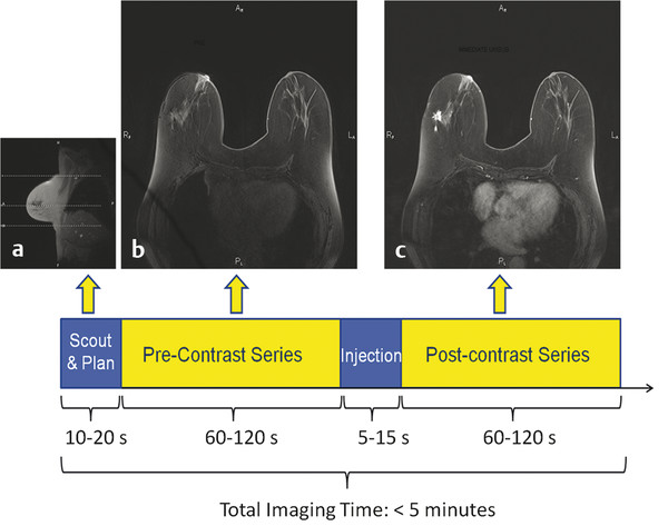
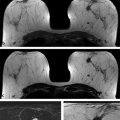
Fig. 5.1 Schematic of abbreviated breast magnetic resonance imaging (MRI) protocol and example images. (a) A sagittal scout view from a three-plane localizer for a 128-slice transaxial acquisition on a 3 Tesla (T) system. The dashed white lines on the scout image indicate the locations of the first, last, and currently displayed slice of a subsequent multiphase T1-weighted series. (b) One of 128 transaxial slices from a 1-minute precontrast acquisition. (c) The corresponding slice from a postcontrast acquisition, displaying a 1.7-cm spiculated invasive ductal carcinoma in the right breast (appearing on the left-hand side of the image). Pre- and postcontrast transaxial 3D acquisitions were identical, with 128 contiguous 1.2-mm thick slices, each acquired with a 487 (phase-encoding, horizontal) × 512 (frequency-encoding, vertical) matrix using a 360 mm × 360 mm field of view, resulting in in-plane pixel sizes of 0.74 mm (phase-encoding) × 0.70 mm (frequency encoding).
5.2 Essential Equipment Requirements for Abbreviated Breast MRI
Essential equipment requirements for abbreviated breast MRI are identical to those for high-quality diagnostic breast MRI. They include the following:
A high magnetic field strength (1.5 T or higher), high homogeneity MRI system.
A dedicated bilateral breast receive or transmit–receive coil with prone patient positioning.
Strong magnetic field gradients with short gradient rise times.
A system capable of obtaining good fat suppression over both breasts.
While these equipment requirements have been described in detail elsewhere for breast MRI, 6, 7, 8 each is described briefly below.
5.2.1 High Magnetic Field Strength, High Homogeneity MRI System
While MRI systems approved by the Food and Drug Administration (FDA) for clinical use have magnetic field strengths ranging from 0.064 up to 3.0 T, systems used for abbreviated MRI should have magnetic field strengths of 1.5 T or higher. There are several reasons for requiring a high-field system. Above about 0.3 T, image SNR per voxel increase approximately linearly with magnetic field strength. 9 Consequently, higher static magnetic field strength (Bo) provides higher SNR per voxel. High SNR per voxel is needed to permit rapid imaging of both breasts with high in-plane spatial resolution and thin slices without losing more subtly enhancing non–mass-like lesions, such as some ductal carcinomas in situ (DCIS).
A second reason for performing breast MRI at high magnetic field strength is to ensure higher static magnetic field homogeneity over the entire imaged volume. High magnetic field homogeneity for breast imaging requires that the static magnetic field strength should remain uniform within about 1 part per million (ppm) across both breasts. At 1.5 T, the resonant frequency of the static magnetic field is about 64 MHz, so uniformity at 1 ppm corresponds to a 64-Hz frequency shift across the entire imaged volume. It is difficult for scanners of magnetic field strengths lower than 1.5 T to maintain a uniform magnetic field at the level of 1 ppm across the volume of both breasts (30–35 cm left to right and posterior to anterior). The main reason for maintaining this high level of magnetic field uniformity is to obtain good fat suppression based on the chemical shift between water and fat over the entire imaged volume, as will be discussed below.
5.2.2 Dedicated Bilateral Breast Coil with Prone Positioning
Dedicated bilateral receive or transmit–receive breast coils have been shown to yield SNR 5 to 10 times that of the body coil ( ▶ Fig. 5.2). When dedicated breast coils are receive-only coils, the radiofrequency (RF) transmit coils are those built into the scanner bore, the same transmit coils used for whole-body imaging or with other receive-only coils, such as spine coils, abdomen coils, and dedicated coils used for most other anatomical regions. When the breast coil is a transmit–receive coil, the breast coil is designed both to send RF signal into the breasts (to excite measurable signals from hydrogen nuclei) and, a short time later, to measure the signals emitted from breast tissues.
Current breast coils, whether transmit–receive or receive-only coils, have multiple receive channel elements. Bilateral breast coils have between two channels (one channel for each breast) and 18 channels. Multichannel coils record received signals from each channel simultaneously using a different amplifier and analog-to-digital converter for each channel. Like other coils, multichannel breast coils must be matched to the data-handling capabilities of the MR scanner hardware and software to simultaneously record and process multiple channels of data.
When a woman has both breasts, bilateral breast imaging is recommended for a number of reasons. 10 First, comparison of both breasts helps identify focal and asymmetric enhancement patterns that may signal breast cancer ( ▶ Fig. 5.3). This helps prevent false-positive interpretations due to physiologic enhancement, which tends to be bilaterally symmetric, especially in premenopausal women and in postmenopausal women on hormone replacement therapy. 11, 12 Second, when a breast cancer occurs, there is about a 3 to 5% chance that breast MRI will detect a mammographically occult breast cancer in the contralateral breast, 13, 14, 15, 16, 17, 18 so it is important to examine both breasts. Third, bilateral breast imaging eliminates some of the artifacts that can occur in unilateral imaging, such as wrap artifacts from the contralateral breast when the field of view (FOV) is set for only a single breast ( ▶ Fig. 5.4). 6
Prone positioning in a dedicated bilateral breast coil helps reduce breast motion and respiratory and cardiac pulsation artifacts, without distorting the breasts. The screened woman is supported in the bilateral breast coil at the sternum, lateral chest, and above and below the coil, with breasts pendent within the coils. Providing mild compression to the breasts without deforming them can further minimize breast motion during imaging and prevent misregistration between pre- and postcontrast scans. Any motion between pre- and postcontrast scans or during scanning can cause blurring of images, motion artifacts, and misregistration artifacts in both subtracted images and the MIP images reconstructed from the volume of subtracted images. Mild compression parallel to the acquisition plane also can help limit the number of slices needed for the screening study. By positioning the patient comfortably and by properly instructing the patient prior to the pre- and postcontrast T1-weighted series pair, rather than after the precontrast scan and just prior to contrast injection, the MR technologist plays an important role in minimizing motion and misregistration. The 3- to 5-minute imaging time of abbreviated breast MRI also should limit patient motion during scanning. Technologists performing either conventional breast MRI or abbreviated breast MRI should be aware of techniques to optimize patient positioning. 19
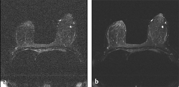
Fig. 5.2 Images of the same slice of the same patient using (a) the body coil as the receiver coil and (b) a dedicated bilateral breast coil as the receiver coil. Note that smaller vessels visible in (b) are obscured in (a) due to excessive image noise.
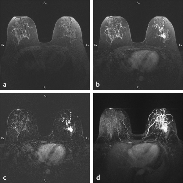
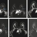
Fig. 5.3 (a) A single precontrast, (b) postcontrast, and (c) subtracted (b minus a) slice in a 3D acquisition in a 41-year-old woman with invasive ductal carcinoma with intraductal component. (a) and (b) were acquired in 3D acquisitions each taking 95 s, with a 340 mm × 340 mm field of view and 448 × 448 matrix, resulting in in-plane pixels of 0.76 mm on a side. Bilateral comparison afforded by transaxial slice acquisition aids differential identification of cancer versus estrogen-related enhancement of normal fibroglandular tissues. (d) Maximum intensity projection (MIP) through all 160 1-mm slices of the subtracted image set, even better revealing the extent of the cancer and the value of bilateral comparison.
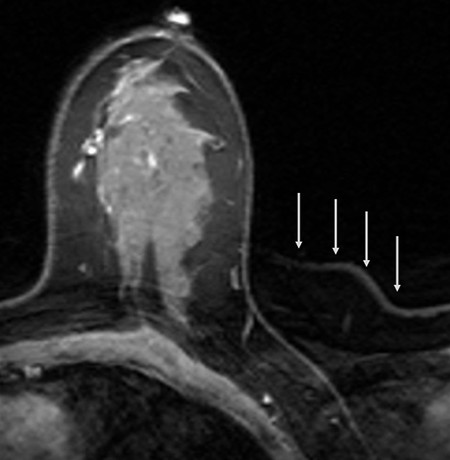
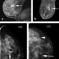
Fig. 5.4 Wrap (or aliasing) artifact of the contralateral breast in a unilateral transaxial acquisition, with phase encoding left to right. Note that the wrap artifact is most apparent outside the imaged breast (arrows), but also wraps across and adds structured noise within the imaged breast.
5.2.3 Strong Magnetic Field Gradients with Short Gradient Rise Times
Magnetic field gradients are required in each perpendicular direction (x, y, and z) to resolve the volume of tissue within the bore of the scanner into individual voxels. Magnetic gradients are turned on and off quickly many times during a pulse sequence series to select a slice or volume of tissue and to resolve signals from a slice into pixels (in 2D acquisitions) or to resolve signals from a volume into voxels (in 3D acquisitions). 6 Two parameters characterize the performance of magnetic field gradients: maximum gradient strength, which determines the maximum change in magnetic field over a given distance along the x, y, or z axis, and gradient rise times, which describe the time interval needed to turn a magnetic field gradient from zero to maximum strength. Magnetic gradient strength helps determine how small voxels can be made, while gradient rise times determine how quickly the pulse sequence that resolves signals into pixels or voxels can proceed. The shorter the gradient rise times, the shorter repetition time (TR) and echo time (TE) can be made. This is especially important in 3D gradient-echo imaging for abbreviated breast MRI, because short TRs and TEs are required to produce strongly T1-weighted images in the limited time available for a full 3D series to be obtained (1–2 minutes). Modern MR scanners have maximum gradient strengths of 40 to 50 mT/m and gradient rise times as short as 200 μs, yielding TR values as short as 4 ms and TE values as short as 1 ms. To obtain adequate spatial resolution over both breasts in 1 to 2 minutes per 3D gradient-echo series, TR needs to be less than 6 ms and TE needs to be less than 3 ms.
5.2.4 Good Fat Suppression over Both Breasts
The question of whether fat suppression is advantageous for abbreviated breast MRI is still open. The abbreviated breast MRI proof-of-concept study conducted by Kuhl et al used bilateral 2D gradient-echo imaging without fat suppression. 1 Through discussions with Dr. Kuhl, I have learned that their 2D non–fat-saturated approach is sometimes helpful in confirming the presence of suspicious lesions by seeing lesion margins, and in particular spiculations, in precontrast series as lower signal areas in a background of bright fat. Most dynamic breast MRI exams performed in the United States, on the other hand, employ 3D gradient-echo imaging with fat suppression. 3, 4, 5, 6, 8 In this approach, lesion margins and spiculations are typically best seen in postcontrast, subtracted, or MIPs of subtracted series. This chapter’s perspective, based on extensive experience with dynamic breast MRI, is that if abbreviated MRI can be shown to be effective using multiplanar 2D gradient-echo imaging acquisitions without fat suppression, as it has by Kuhl et al, 1 then it should be at least as effective using appropriate 3D gradient-echo acquisitions with fat suppression. The preliminary abbreviated MRI studies using a 3D fat-suppressed approach seem to support this view, at least as far as sensitivity to breast cancer is concerned. 3, 4, 5 The effect on specificity of performing abbreviated MRI using 3D, fat-suppressed acquisition techniques on a high-risk or intermediate-to-high-risk cohort remains to be seen.
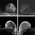
The inclusion of fat suppression in the pre- and postcontrast T1-weighted pair in abbreviated breast MRI improves the conspicuity of enhancing lesions in postcontrast images and reduces confounding background noise and artifacts that can mimic or mask enhancing lesions in subtracted images and MIP images reconstructed from the set of subtracted images ( ▶ Fig. 5.5). When pre- and postcontrast images are acquired without fat suppression, misregistration of fat between the two series can result in residual fat signals in subtracted and MIP images that can simulate enhancing lesions, especially non–mass-like lesions, leading to false-positive findings. In addition, residual fat signal in subtracted images adds structured noise that can mask detection of subtle non–mass-like lesions characteristic of DCIS, leading, in some cases, to false-negative interpretations.
Unfortunately, there are no clinical studies that compare similar contrast-enhanced breast MRI techniques with and without fat suppression, in either dynamic breast MRI or abbreviated breast MRI. This is due, at least in part, to the necessity in such studies to image each study volunteer twice, once with and once without fat suppression, each time injecting contrast agent.
The next section describes details of the gradient-echo pulse sequence needed to maximize enhancing lesion conspicuity in abbreviated breast MRI.
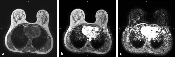
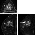
Fig. 5.5 (a) Precontrast and (b) postcontrast scans acquired without fat saturation and with the body coil as the receiver coil, rather than a dedicated bilateral breast coil. (c) The subtracted image (b minus a) shows artifacts in both breasts due to misregistration of pre- and postcontrast scans, making it difficult to distinguish enhancing lesions from background noise due to misregistration of unsuppressed fat between pre- and postcontrast series.
5.3 Essential Abbreviated Breast MRI Screening Exam
The essential elements of an abbreviated breast MRI exam are as follows:
Identical pre- and postcontrast T1-weighted gradient-echo acquisitions, each of 1- to 2-minute duration.
Inclusion of all breast tissue.
In-plane spatial resolution (pixel size) of 1 mm or less.
Acquired slice thickness of 3 mm or less.
Adequately high SNR to detect small (1–2 mm diameter) vessels in MIP reconstructed images.
Each of these essential elements is discussed below.
5.3.1 Identical Pre- and Postcontrast T1-Weighted Gradient-Echo Acquisitions, Each of 1- to 2-Minute Duration
T1-weighting is used in contrast-enhanced breast MRI, as in other clinical applications of gadolinium (Gd) based contrast agents, because Gd-chelates, while shortening both T1 and T2 (or T2* in gradient-echo series), cause a greater change in T1 than in T2 or T2*. 20 Gradient-echo imaging is used because it is most efficient in obtaining strong T1-weighting, while permitting high-resolution imaging. Gradient-echo imaging achieves strong T1-weighting by using a short TR value, a very short TE value, and a low flip angle that is matched to the TR value to obtain maximum SNR per unit time or maximum contrast-to-noise ratio (CNR) between lesion and background tissues per unit time. 6 For 3D (volume) acquisitions, signal is acquired from a volume of tissue in position space and phase encoded to separate signal into two perpendicular directions, with frequency encoding separating signal in the third perpendicular direction. This can be thought of as filling a volume of signal data in 3D spatial frequency (or k-) space. A 3D Fourier transform (3DFT) is used to convert the signals collected in 3D k-space into individual voxels in 3D position space. This collection of signal from an entire volume of data, rather than just single planes of data as is done in 2D or planar imaging, adds efficiency to the 3D technique. Extremely short TR values are required in 3D imaging, however, to keep the scan times for the pre- and postcontrast T1-weighted series short, under 2 minutes per series in abbreviated breast MRI. For 3D acquisitions where TR values are extremely short (under 10 ms), gradient-echo flip angles are usually 10 to 15 degrees. 6
For 3DFT imaging, total acquisition time is T = (TR)(Npe)(Nacq)(Nslices), where TR is the pulse sequence repetition time, Npe is the number of in-plane phase-encoding steps (to resolve signal into voxels along one in-plane direction, the phase-encoding direction), Nacq is the number of times each phase encoding step is repeated (which is almost always set to 1 in 3DFT imaging), and Nslices is the number of acquired slices within the 3D volume, which in 3DFT imaging is the number of phase-encoding steps used to separate the 3D volume into a second perpendicular direction, in this case the slice-select direction ( ▶ Fig. 5.6). Frequency encoding applied during signal acquisition is used to separate the 3D volume into the third perpendicular direction, the frequency-encoding direction, but fortunately does not require an additional time factor to do so. In 2DFT (planar) imaging, Nslices is automatically set to 1 in the Ttotal formula, TR and flip angle are increased, and a multislice approach is used. Because in 3D imaging the additional factor, Nslices, is large, typically 80 to 160 in breast MRI, very short TR values are needed in 3DFT imaging to achieve reasonably short total scan times per series. For example, a typical 3D acquisition has TR = 5 ms, Npe = 320 (the number of matrix elements in the phase-encoding direction), Nacq = 1, and Nslices = 120, so Ttotal = (5 ms) (320) (1) (120) = 192,000 ms = 192 s, or 3 minutes, 12 s. This is still too long for a single pre- or postcontrast series in abbreviated breast MRI, so additional techniques compatible with 3DFT gradient-echo acquisitions are needed to further shorten acquisition times. These include the use of parallel imaging, partial-Fourier acquisitions, and slice interpolation, each of which is described below.
3DFT (volume) acquisitions have advantages over 2DFT (planar) acquisitions. One is a signal-to-noise advantage because 3DFT acquisitions collect signal from an entire volume of tissue that includes both breasts during each signal measurement, instead of from just a single plane of tissue as occurs in 2DFT imaging. This makes 3DFT acquisitions more efficient, but at the expense of requiring more total scan time (by the factor Nslices) to resolve the entire 3D volume into individual voxels. 2DFT acquisitions require resolving only a single preselected plane into individual voxels, using phase encoding to resolve signals in one in-plane direction and frequency encoding to resolve signals in the other perpendicular in-plane direction.
A second advantage of 3DFT acquisitions is that they always subdivide signals in the slice-select direction into contiguous slices with rectangular slice profiles (meaning that all tissues within each slice contribute to the measured signal), while 2DFT imaging typically has small gaps between individual slices and measured signals have Gaussian slice profiles (where signal is predominantly measured from the center of each slice and the signals from slice edges are reduced or lost), as shown in ▶ Fig. 5.7. A third advantage of 3DFT acquisitions is that with thin slices, isotropic voxels (meaning voxels with the same dimension in all three perpendicular directions) or nearly isotropic voxels can be acquired. This in turn enables orthogonal plane or MIP reconstructions of subtracted image data in virtually any orientation without loss (or in the case of nearly isotropic voxels, with only minor loss) of spatial resolution, which can permit better visualization of enhancing lesion margins. 2D or 3D acquisitions with thicker (e.g., 1.5-mm or greater) slices typically are limited to reconstruction of MIP image projections along the slice-select direction to avoid the degradation of spatial resolution that occur in other planar or MIP projections, due to slice thickness significantly exceeding in-plane spatial resolution.
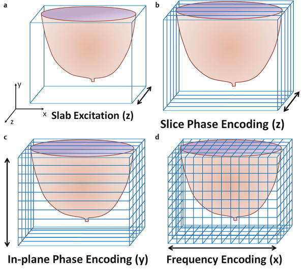
Fig. 5.6 Schematic illustrating 3D (volume) acquisition of slices in the transaxial (z-) plane. (a) The slice-select gradient (along the z-axis for a transaxial acquisition) is turned on to select a slab or volume of tissue to be excited by the radio frequency pulse transmitted into the patient after the patient’s breasts are placed as closely as possible to the isocenter of the magnet. (b) In a series of pulse sequence repetitions with different amounts of phase encoding applied along the z-direction, the excited slab is resolved into slices within the volume. The number of different slices resolved equals the number of slice phase-encoding steps. (c) For each slice phase-encoding step, the pulse sequence is repeated with a different in-plane phase-encoding gradient to resolve the volume of tissue into different planes in the in-plane phase-encoding direction, y. The number of in-plane phase-encoding views collected for each slice phase encoding equals the number of matrix elements in the y-direction. (d) During each signal readout, a frequency-encoding gradient is turned on in the third (in this case, x-) direction to resolve the volume into different voxels along the third orthogonal (x-) direction. The number of different time points at which signal is measured during each signal readout equals the number of matrix elements along the x-direction. The total imaging time for a 3D pulse sequence acquisition is Ttotal = (TR) (Npe) (Nacq) (Nslices), where TR is the gradient-echo pulse sequence repetition time, Npe is the number of in-plane phase-encoding steps (the number of matrix elements in the in-plane phase encoding direction), Nslices is the number of slices acquired within the 3D volume, and Nacq is the number of times the entire process is repeated, which is usually set to 1 in 3DFT acquisitions.
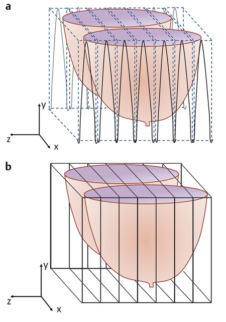
Fig. 5.7 Schematic of the slice profiles in (a) 3DFT and (b) 2DFT acquisitions. (a) In 3D or volume acquisitions, slice profiles are rectangular and slices are always acquired contiguously. As a result, signals are measured uniformly from all tissues in each slice. (b) In multislice 2D or planar acquisitions, slice profiles are Gaussian, as shown by the solid black curves, and more signal comes from the center of each slice than from the edges. Often, 2D acquisitions are done with small gaps between slices, shown by the dotted vertical lines, to reduce cross-talk between slices in multislice acquisitions, which further reduces signal measured per slice.
5.3.2 Methods to Speed 3D Gradient-echo Pulse Sequence Acquisitions
Parallel Imaging
To save additional time in either 2D or 3D acquisitions, parallel imaging can be used, assuming the scanner has the software and appropriate breast coils. This is apparent on the technologist scan menu. Many 3D gradient-echo series have parallel imaging options and some permit adjustment of the parallel imaging acceleration factor (AF). For example, if an AF of 2 is selected, scan time will be cut nearly in half for the same coverage, spatial resolution, and slice thickness. Parallel imaging does this by acquiring multiple segments of data simultaneously, speeding the data acquisition process. 21 This acceleration of data collection can occur either in physical space (for instance, one segment of signal data being acquired on the left breast, while the other segment is simultaneously acquired on the right breast) or in k-space, where, for AF = 2, every other line of signal data in k-space is sampled and intervening lines of data are interpolated. In either case, the sensitivity profiles of individual receiver coil elements are measured on that patient (which takes a small amount of additional time) to compensate for the simultaneously acquired or missing data and to enable reconstruction of parallel-acquired data into images. One prerequisite to parallel imaging is that the receiver coil must have at least as many channels as the AF. So for an AF of 2, the breast receiver coil must have at least two channels, but could also have a higher number of channels that get combined into two data segments.
In practice, parallel imaging with too high an AF leads to excessive artifacts in the resulting images ( ▶ Fig. 5.8). Typically, at 1.5 T, AF is not set to be greater than 2, while at 3.0 T, the AF is not set to be greater than 3. Even with AF = 2, the time for a full 3DFT acquisition would be reduced from 192 s (in the example of 3DFT image acquisition described above) to 81 to 110 s, a range that would be acceptable for each pre- or postcontrast series in an abbreviated breast MRI exam. The reason that a range of acquisition times is stated for an AF of 2 is that some manufacturers acquire the calibration scan that measures the sensitivity profiles of each coil channel as a separate pulse sequence when parallel imaging is prescribed, while other manufacturers acquire the calibration scan within the parallel imaging sequence itself. In either case, there is a small amount of additional time needed beyond the time estimated by dividing the original series scan time by the AF.
While reducing scan time by a factor nearly equal to the AF, there is an SNR penalty for using parallel imaging. SNR is reduced by a factor equal to the square root of the AF, so for AF = 2, SNR is reduced by a factor of 1.41, resulting in an SNR that is approximately 71% of that without using parallel imaging ( ▶ Fig. 5.8). For AF = 3, SNR would be reduced to approximately 58% of that without parallel imaging, although this degree of SNR loss would be compensated by the nearly doubled SNR at 3.0 T compared to 1.5 T, all other acquisition parameters being equal.
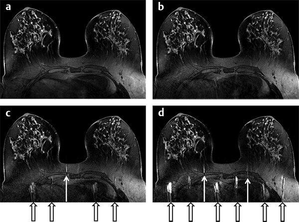
Fig. 5.8 A single slice from 3.0-T transaxial bilateral 3D T1-weighted breast images acquired without (a) and with increasing acceleration factors in parallel imaging (b–d). In each case, an entire volume was acquired covering both breasts, with identical spatial resolution and breast coverage. (a) Without parallel imaging, the 3D volume series took 102 s. (b) With AF = 2, the 3D series took 57 s. (c) With AF = 3, the 3D series took 42 s. (d) With AF = 4, the series took 34 s. Note the increased number and strength of artifacts (pointed out by the black and white arrows) and decreased pixel signal-to-noise ratio as acceleration factor is increased, but without loss of spatial resolution.
Related posts:
 Current Clinical Evidence on Abbreviated Breast Magnetic Resonance Imaging
 Abbreviated Breast Magnetic Resonance Imaging Protocols and Clinical Implementation
 Introduction to Abbreviated Breast Magnetic Imaging
 Technical Aspects of Abbreviated Breast Magnetic Resonance Imaging: The Original Approach
 Magnetic Resonance Imaging-Guided Biopsy Techniques
 Interpretation Guidelines
Stay updated, free articles. Join our Telegram channel

Full access? Get Clinical Tree


