Fig. 3.1
Uptake of the NK1 receptor ligand [11C]R116301 in a normal volunteer with (left) a total uptake image (60–90 min after injection) and (right) a parametric image on non-displaceable binding potential (BPND) representing specific signal only
3.2 Principles of Modelling
As mentioned above, PEt allows for accurate measurements of regional tissue radioactivity concentrations. The purpose of a PET study, however, is to obtain quantitative values of parameters that characterize a physiological, biochemical or pharmacokinetic process. In other words, a tracer kinetic model, describing the process under study, is required to translate the measurements of radioactivity into quantitative values of these biological parameters. Although other models are available, in practice, all PET studies are analysed using compartment models (Gunn et al. 2001). These compartments not necessarily are distinct anatomical compartments but a convenient way to describe different kinetic “states” of the tracer. The most common models are single- and two-tissue compartment models (Fig. 3.2).
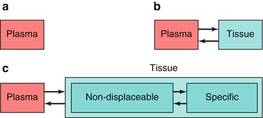

Fig. 3.2
Structure of compartment models with (a) no-, (b) one- and (c) two-tissue compartments
The simplest model, a zero-tissue compartment model (Fig. 3.2a), can be used for a blood volume tracer, such as [15O]CO or [11C]CO (Phelps et al. 1979a). CO binds to red cells and remains in the vascular space (no tissue compartment). As CO binds to red cells, a correction for the small- to large-vessel haematocrit ratio is needed to obtain values of blood volume (Lammertsma et al. 1984). This clearly illustrates that one should always be aware of underlying assumptions in the model, as differences in capillary and large-vessel haematocrit could easily be overlooked.
A more common model is the single-tissue compartment model (Fig. 3.2b). In this case, the tracer is taken up by tissue, but it has either no further interactions within tissue (e.g. [15O]H2O; Frackowiak et al. 1980) or its kinetics are such that no additional tissue compartments can be identified (e.g. [11C]flumazenil; Koeppe et al. 1991). In a two-tissue compartment model, a second-tissue compartment is introduced with additional rate constants to describe exchange of tracer between the two tissue compartments (Huang et al. 1980). In general, the first compartment represents free and non-specifically bound tracer and the second compartment metabolized (e.g. [18F]FDG; Phelps et al. 1979b) or bound (e.g. [11C]raclopride; Farde et al. 1989) tracer.
Since the introduction of quantitative PET, there has been confusion about the nomenclature of both the models themselves and the parameters associated with them. Initially, single-tissue compartment models were referred to as either single (tissue) or two (blood and tissue) compartment models, and a similar problem existed for two-tissue compartment models. Fortunately, in recent years, there is consensus to classify models according to the number of tissue compartments involved. More importantly, a multitude of symbols has been used to indicate parameters associated with these models, in particular volume of distribution and binding potential. To provide clarity, in 2007, consensus was reached about the nomenclature related to reversibly bound ligands (Innis et al. 2007), and, wherever possible, this nomenclature will be used here.
3.3 Single-Tissue Compartment Model
As mentioned above, the single-tissue compartment model (Fig. 3.3) can be used for tracers where no second-tissue compartment is present or identifiable. The differential equation describing this model is given by
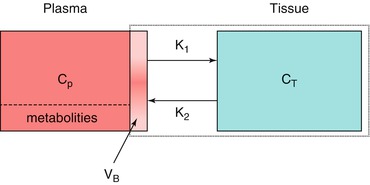

where C T and C P are tissue and arterial plasma concentrations as function of time t and K 1 and k 2 rate constants for influx into and efflux out of tissue, respectively. This differential equation provides a mathematical description of the fact that the rate of change of the concentration in tissue depends on the balance between total rate of influx and total rate of efflux. The rate constant K 1 depends on two components according to

where E is the first-pass extraction fraction and F blood flow (perfusion). It has been well documented that E itself depends on F according to (Renkin 1959; Crone 1963)

where PS represents the permeability surface area product. This equation illustrates that E is constant for flow values that are small compared with PS. For higher flow values, however, E starts to decrease, reflecting the phenomenon that the chance of a molecule to cross the capillary wall reduces if flow increases.

Fig. 3.3
Schematic diagram of the general single-tissue compartment model. C P and C T represent arterial plasma and tissue concentrations, K 1 and k 2 influx and efflux rate constants and V B blood volume within the PET region

(3.1)

(3.2)

(3.3)
An important parameter, independent of the actual model, is the volume of distribution V T, which is the ratio of tissue and plasma concentrations under steady-state conditions, i.e. at equilibrium when both concentrations are time independent:


(3.4)
At equilibrium, the single-tissue compartment model reduces to:


(3.5)
Rearranging results in:


(3.6)
In other words, for the single-tissue compartment model, it follows that:


(3.7)
The general solution of Eq. 3.1, with or without Eq. 3.7, is

where ⊗ represents the convolution operation.

(3.8)
In practice, a PET scanner does not only measure uptake in tissue but rather total uptake in a region of interest (ROI) or voxel. In other words, intravascular activity should also be taken into account. Consequently, the concentration measured by the PET scanner is given by:

where V B represents (fractional) blood volume, C A(t) arterial whole blood concentration as function of time and C T(t) is given by Eq. 3.8.

(3.9)
3.4 Principles and Practice of Quantification
Equation 3.9 illustrates a couple of basic principles of quantification of PET studies. Firstly, it clearly illustrates that activity is delivered to tissue through the circulation, and therefore, for full quantification, the arterial plasma concentration C P(t) needs to be measured as function of time. If the tracer is metabolized and (ideally) its radioactive metabolites do not cross the blood-brain barrier, C P(t) represents the time-activity curve of parent tracer only. In other words, in general, the metabolite-corrected arterial plasma curve is needed. Secondly, although C P(t) provides input to tissue, intravascular activity is a mixture of parent tracer, its radiolabelled metabolites and indeed tracer (or metabolites) bound to blood cells. Consequently, as a second input function, the non-metabolite-corrected arterial whole blood curve C A(t) is needed. Thirdly, the convolution in Eq. 3.9 indicates that the tissue concentration C T(t) does not depend on the instantaneous C P(t) value but rather on its history. This is just a mathematical representation of the fact that tissue clearance is not instantaneous. Finally, apart from the measured variables C P(t), C A(t) and C PET(t), Eq. 3.9 contains two-tissue-related unknown parameters K 1 and V T. With two unknown parameters, it will be clear that it is not possible to solve Eq. 3.9 using a single (static) scan (i.e. Fig. 3.1b cannot be derived from Fig. 3.1a without additional information).
To derive quantitative values of both K 1 and V T, dynamic scanning is required. In contrast to most diagnostic procedures where a static scan is acquired sometime after tracer injection, in a dynamic scanning protocol, the patient is first positioned within the scanner. With the patient in the scanner, the tracer is injected, and, at the same time, a (dynamic) scan is started with an overall length that is dictated primarily by the kinetics of the process/tracer under study. To date, most scanners acquire data in list mode (each event has a time stamp), but during data processing counts are binned into successive time frames. Reconstruction of these frames provides a series of images as function of time. From these frames, time-activity curves (i.e. C T(t)) can be generated at either a voxel or a region of interest (ROI) level.
C A(t) can be obtained by continuous arterial blood sampling (Boellaard et al. 2001) during scanning. Additional manual arterial blood samples are needed to obtain C P(t). These samples are needed to obtain plasma to whole blood ratios and parent fractions, both as function of time. Curves are fitted to both manual data sets, and C A(t) is multiplied with both curves, resulting in C P(t). When all data are available, a voxel or ROI time-activity curve C T(t) can be fitted for K 1 and V T (or k 2) using the operational equation (Eq. 3.9), together with input functions C P(t) and C A(t) and standard non-linear regression techniques (Cunningham 1985).
3.5 An Example: Measurement of CBF Using [15O]H2O
As mentioned earlier, the single-tissue compartment model can be used for tracers that enter tissue but have no further interaction within that tissue. Such a tracer is ideal for measuring tissue perfusion, and the best example is [15O]H2O (Lammertsma et al. 1989). Water is freely diffusible in the brain, at least at normal and reduced flow values. In addition, it is metabolically inert (no interaction in tissue). Being freely diffusible means that the first-pass extraction fraction is 100 %, i.e. E = 1. From Eq. 3.2, it follows that K 1 = F and, from Eq. 3.7, k 2 = F/V T where, in the brain, F represents cerebral blood flow (CBF).
For perfusion, not the arterial plasma concentration is relevant but rather the whole blood concentration. For water, this makes little difference, as concentrations are nearly the same. In this case, V T = C T/C A (at equilibrium), and it can be seen that the volume of distribution is identical to the partition coefficient of water.
As the partition coefficient of water is close to one (Herscovitch and Raichle 1985; Lammertsma et al. 1992), the venous concentration of [15O]H2O will be similar to the tissue concentration, and it will not be possible to separate these from each other. In other words, the fractional blood volume in Eq. 3.9 is essentially the fractional arterial blood volume V A, which in the brain is in the order of about 1 % (except in the vicinity of large arteries). In practice, V A is left out of the equation, as it reduces precision (one more parameter to fit) and it has been shown that fitted F values are essentially the same when V A is included or excluded. Therefore, for [15O]H2O, Eq. 3.9 reduces to:


(3.10)
A schematic diagram showing the principles of obtaining F and V T from measured tissue and arterial blood time-activity curves is shown in Fig. 3.4.
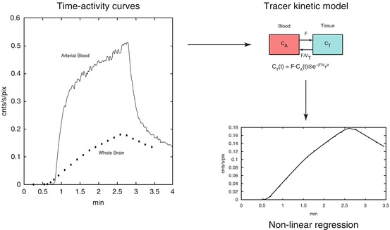

Fig. 3.4
Schematic diagram showing the fitting process, in this case, for flow F and volume of distribution V T using [15O]H2O as tracer. The left panel shows arterial blood and whole brain [15O]H2O time-activity curves. The tissue curve is then fitted using the arterial whole blood curve as input function together with the model shown in the right upper panel. The best fit is shown in the lower right panel. Note that additional parameters are needed to account for delay and dispersion of the arterial input function
3.6 Two-Tissue Compartment Model
The most widely used tracer kinetic model is the two-tissue compartment model (Fig. 3.5), as it is used for both metabolism and neuroreceptor studies. The standard (reversible) two-tissue compartment model contains four rate constants (K 1 to k 4), but for tracers that are trapped in the final compartment, it reduces to an irreversible two-tissue compartment model in which k 4 = 0.
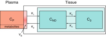

Fig. 3.5


Schematic diagram of the two-tissue compartment model. C P, C ND and C S represent arterial plasma, non-displaceable tissue and specific tissue concentrations; K 1 to k 4 rate constants characterizing transport between compartments; and V B blood volume within the PET region
Stay updated, free articles. Join our Telegram channel

Full access? Get Clinical Tree


