Treatment Planning
CHAPTER 8.A PRINCIPLES OF SYSTEMS AND OPTIMIZATION
Hanne M. Kooy
Alexei Trofimov
Martijn Engelsman
Alfred R. Smith
Robert Wilson in 1946, while directing the design of the second proton cyclotron at Harvard University, recognized the clinical potential of the high-density ionization profile of the proton Bragg peak. (The first Harvard cyclotron was dismantled in 1943 and moved to Los Alamos, also under Wilson’s direction, to support the Manhattan project.) Fifteen years later, this clinical potential was achieved at the Harvard Cyclotron Laboratory using the second proton cyclotron. At that time, as was the case with other such facilities around the world, research cyclotrons had become obsolete and some had been converted for clinical purposes. Most cyclotrons, due to energy limitations, could only be effectively used in the treatment of eyes, which proved to be one of the success stories of proton radiotherapy with local cure rates near 98%. The second Harvard cyclotron, fortuitously, had a sufficiently high energy of 165 MeV (equal to a penetration depth, range, of 18 cm in water) to be of clinical utility in several clinical sites. In contrast, the first Harvard cyclotron had a beam energy of 12 MeV, equal to a range of only 0.17 cm in water!
The early clinical use of protons was promoted for neurosurgical treatments by Kjellberg and Leksell.1,2 This early clinical use was very much enabled by two factors that compensated for the absence of now readily available technologies. First, the absence of volumetric imaging modalities only enabled treatments in those sites, notably in the cranium, where planar x-rays provided target identification with sufficient geometric precision to achieve a benefit from proton beams. Second, the simple mechanical manipulation of proton beams, without the use of modern electronic controls, sufficed to create clinically relevant fields. These mechanical manipulations produced proton spread-out Bragg peaks (SOBP) fields that were dosimetrically uniform in the lateral and depth dimensions and that could be constrained by an aperture and range-compensator to achieve accurate lateral and distal target dose conformation respectively.
Such SOBP field delivery techniques, albeit more automated, are still the standard treatment choice for the vast majority of patient proton treatments. It is expected that dynamically, that is, under full electronic control, scanned and modulated proton beams will gain rapid acceptance when available in the clinical proton centers. Nevertheless, SOBP field treatments will remain the standard for the near future.
Fundamentally, the clinical utilization of proton beams was advanced by the introduction of volumetric imaging modalities, the ability to process those modalities in the treatment planning process, the early clinical successes and clear dosimetric advantages of proton radiotherapy, as well as the parallel advances, and justification, in photon radiotherapy for increased precision in dose and target localization. All these factors combined to make proton radiotherapy a viable treatment strategy which has permitted the technology to migrate from the laboratory setting to the hospital. The current appeal for clinical facilities is very high and is primarily limited by the high start-up costs of a facility and the, as of yet, limited operational expertise in the radiotherapy community. It is assumed that the operational costs, apart from maintenance, are comparable to that of a modern radiotherapy clinic, which also aims to achieve the highest precision in dose delivery commensurate with the clinical need.
SCATTERED PROTON FIELDS
Beam Production
A proton clinical facility will have a proton producing accelerator (a cyclotron or synchrotron), an energy selection system to produce a proton beam of the desired energy, a magnetic beam line to transport the beam, a delivery system to produce the patient-specific treatment field, and a positioning system to either move the beam, the patient, or both, to achieve the desired beam position with respect to the patient. Figure 8A.1 shows an example of a gantry-based treatment room, with an isocentric gantry and a six-axes patient positioner, and an example of a fixed beam line where positioning is achieved solely by a five-axes patient positioner.
The energy selection system is an essential component as it changes the proton beam energy, as produced in the accelerator at some typically fixed energy, to the desired prescription energy. Of note, for heavy charged particles, energy is equated directly to range—changes in energy therefore equate to changes in depth. The energy can be changed simply by inserting material in the beam, which reduces the range by the amount of material water-equivalent thickness along the beam direction. This simple mechanical manipulation of the beam energy allows precise changes of the depth of penetration. Insertion of material, however, does not change the intensity of the beam. This is the reverse of the effect of material inserted in a photon beam where the material does not affect the energy spectrum (to a good approximation in clinical beams) but does attenuate the intensity. The energy selection system is typically distributed over several subcomponents. For a cyclotron, one part is external as the cyclotron produces a proton beam of constant and highest energy only. The beam energy therefore requires significant reduction beyond what is achievable or practical in the delivery system. In contrast, a synchrotron produces, in theory but not in typical practice, a beam of arbitrary energy and transports the extracted beam directly to the delivery system. In practice, the locations where the field-specific proton beam energy is adjusted vary. This impacts the design of the beam line and delivery system and even the operation of the facility. In one extreme, for example, the energy is arbitrary before entry into the beam line and the beam line must therefore allow for continuous variation in its magnetic fields to maintain the proper orbit for the proton beam, whereas the delivery system only needs to provide the ability to modulate, that is, spread out, the energy. On the other extreme, the energy is constant, or limited to a set of discrete values, which simplifies the beam line control requirements, but now requires the delivery system to shift the energy to the desired in-patient penetration range as well as implement range modulation.
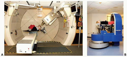 Figure 8A.1 A: A gantry treatment room, (B) a fixed beam line treatment room, both at the Francis H. Burr Proton Therapy Center at the Massachusetts General Hospital (MGH). The gantry room has an isocentric gantry (SAD ˜230 cm) and a six axis of freedom patient positioner. The most prominent visible feature is the nozzle assembly (see Fig. 8A.2 for the set of components that are typically housed in the nozzle) attached to the gantry. The patient positioner, in this gantry, has 6 degrees of motion including extended lateral motion. The fixed beam line room (used for stereotactic treatments) depends solely on the 5 degrees of freedom patient positioner to orient the patient with respect to the beam. Specifically, the patient can be rotated 360 degrees around the body axis and allows the beam to be oriented at arbitrary position in the upper cranial hemisphere. The gantry room equipment is built by IBA Ltd. (Louvain la Neuve, Belgium); the fixed beam line equipment is designed and built by MGH engineering staff. |
For the purposes of the clinical production and use of spread-out Bragg peak, SOBP, fields, we need only consider that the delivery system, referred to here as the nozzle, accepts a pristine, that is, monoenergetic, proton beam of a given energy delivered to the nozzle by the beam line. The pristine peak is very narrow in depth, with a typical
90-90% (of maximum dose) width of the Bragg peak of approximately 0.4 cm and has a small diameter on the order of 1.0 cm or less. This narrow peak is, by itself, not clinically useful. The nozzle therefore manipulates this pristine proton beam and produces a proton beam of energy equal to the desired range in the patient, flattens the beam in the lateral extents, and modulates the pristine proton beam in energy and intensity to achieve a uniform depth-dose for the extent of the target volume along the beam axis.
90-90% (of maximum dose) width of the Bragg peak of approximately 0.4 cm and has a small diameter on the order of 1.0 cm or less. This narrow peak is, by itself, not clinically useful. The nozzle therefore manipulates this pristine proton beam and produces a proton beam of energy equal to the desired range in the patient, flattens the beam in the lateral extents, and modulates the pristine proton beam in energy and intensity to achieve a uniform depth-dose for the extent of the target volume along the beam axis.
A modern scattering nozzle (see Fig. 8A.2) has a range-modulation system, consisting of rotating range-modulator wheels (see Fig. 8A.3), optional range-shifter plates to range-shift the SOBP dose distribution to the desired clinical range in patient, scattering filters to flatten the field in the lateral dimensions, dose monitor ionization chambers and other diagnostic devices, and an assembly to mount the patient-field-specific aperture and range-compensator. In general, these components are standard but their arrangement is not. Nozzles are highly individual in their design and proton equipment has certainly not achieved the uniformity of design and use of the modern photon LINAC. In the examples in the following text, therefore, the nozzle is characterized only by the intended purpose, and not explicit design.
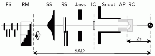 Figure 8A.2 A hypothetical, not to scale, double-scattering nozzle with relevant beam modifying components. These are (from beam entry at left to isocenter at right), a set of lead foils (FS) to adjust the beam scattering as a function of range, a rotating rangemodulator wheel (RM) to continuously, as a function of rotation angle, change the pristine peak range, a second scatterer (SS) used in conjunction with the FS and RM to create a flat field, a set of range-shifter plates (RS) to change the overall energy in the nozzle to the desired range in patient, a set of X and Y jaws to limit the proton field, a reference ionization chamber (IC) system for monitor unit and other field measurements, a snout assembly to mount and position the patient-field-specific aperture (AP) and range-compensator (RC) at the required distance (Zs) from isocenter. All components affect the energy, and the setting of an individual component therefore affects the other components. In general, the overall settings of components are a nontrivial function of the nozzle control system. The range-shifters RS are required if the energy at the nozzle entrance is limited to a set of discrete values at intervals beyond the clinical resolution for range. The range-shifters have thicknesses that vary from the clinical resolution required (e.g. 0.1 cm in water) up to the maximum interval (say 4.0 cm) between energies at the nozzle entrance in values that double between each range-shifter. In our example, the set would require range-shifters of 0.1, 0.2, 0.4, 0.8, 1.6, and 3.2 cm, which in combination create any range-shift between 0.1 to 6.5 cm in steps of 0.1 cm. The source-to-axis distance (SAD) is typically close to the first scattering component, here the RM. The jaws in scattering nozzle serve to reduce proton exposure to materials close to the patient and hence to reduce neutron production in those materials closer to the patient. The jaws have no field-shaping role. |
Scattered Proton Fields
Figure 8A.4 shows a typical SOBP depth-dose along the beam central axis together with the depth-dose curves of the constituent individual pristine Bragg peaks which, in summation and considering their relative amplitude as indicated, produce the SOBP depth-dose. The SOBP depth-dose is specified in terms of range (R), modulation (M) and prescription dose to the 100% plateau. The range R and modulation M are defined here at the 90% dose levels, as is the most common but somewhat arbitrary definition. These parameters are produced in the treatment planning process for each treatment field. If the energy at the nozzle entrance is not continuously variable, range-shifters (labeled RS in Fig. 8A.2) are required to shift the desired SOBP to the prescription range R by inserting the required material between the entering beam and the patient. The proton beam is modulated in intensity and range by rotating modulator wheels. Such wheels have range-shifting thicknesses varying as a function of rotation angle. Typically, thickness is constant for an angular segment, and a wheel has several angular segments of increasing thickness. The thickness sets the pristine peak position equal to the range at nozzle entrance minus that thickness, whereas the width of the angular segment sets the beam-on time at that range position. The combination of thicknesses for various segments produces the set of desired pristine peaks of the correct intensity. Figure 8A.3 shows a rangemodulator wheel originally used at the Harvard Cyclotron Laboratory and a modern, more compact, version. The original production of SOBP fields required one wheel, approximately, per modulation width. The modulation width, after all, is hard-coded into the wheel in terms of the set of angular segments and thicknesses and is equal to the maximum thickness on the wheel, whereas the range incident on the wheel can be varied. A single wheel can therefore produce an SOBP of variable range R but of fixed modulation width M. The use of modern beam control systems extends the applicability of a modulator wheel to variable modulation widths. Given a range-modulator wheel with a maximum modulation width M, one can achieve modulation width less than M by turning off the beam before the wheel has completed a rotation and turning the beam on when the rotation returns to its start position. This permits the exclusion of those pristine peaks that contribute to the SOBP depth-dose beyond the desired modulation width (Fig. 8A.4).
The SOBP dose distribution is further constrained by an aperture, typically constructed from brass, to the beam’s eye view projection of the target. The aperture thickness must exceed the SOBP range by approximately 2 cm to ensure that the proton beam, always at full intensity but diminishing energy, does not traverse the blocked area.
The aperture therefore is functionally identical to a photon beam block. The SOBP dose distribution is also constrained in the depth dimension by a range-compensator to yield a distal dose falloff that conforms to the distal target-volume surface with respect to the beam central axis. The function of the range-compensator is unique to charged particles. The properties of the SOBP, finite range in the patient and a flat dose profile of variable width to fit the target volume extent, combined with an aperture and range-compensator yields a treatment field with a high degree of conformality and dose uniformity to the target volume even for a single treatment field. Therefore, a single proton field can be used to provide complete target volume coverage during a single course of treatment. The effect of a range-compensator is illustrated in Figure 8A.5. Observe that the effect of the range-compensator is solely to locally shift the isodose distribution without, to first order, perturbing the dose intensities.
The aperture therefore is functionally identical to a photon beam block. The SOBP dose distribution is also constrained in the depth dimension by a range-compensator to yield a distal dose falloff that conforms to the distal target-volume surface with respect to the beam central axis. The function of the range-compensator is unique to charged particles. The properties of the SOBP, finite range in the patient and a flat dose profile of variable width to fit the target volume extent, combined with an aperture and range-compensator yields a treatment field with a high degree of conformality and dose uniformity to the target volume even for a single treatment field. Therefore, a single proton field can be used to provide complete target volume coverage during a single course of treatment. The effect of a range-compensator is illustrated in Figure 8A.5. Observe that the effect of the range-compensator is solely to locally shift the isodose distribution without, to first order, perturbing the dose intensities.
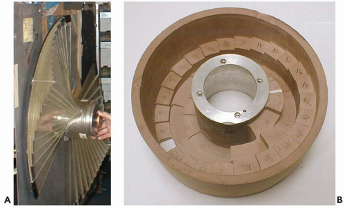 Figure 8A.3 A: A range-modulation wheel, or “propeller,” as used for clinical treatments at the Harvard Cyclotron Laboratory; (B) a range-modulation wheel used in the IBA Ltd. (Louvain la Neuve, Belgium) nozzle. The propeller consists of varying thickness of polystyrene with varying angular widths. The combination of width and thickness determines how much a particular pristine Bragg peak created from the beam incident on the propeller contributes to the spread-out Bragg peak (SOBP). In general, a large set of such propellers was needed to accommodate the variety of SOBPs as set by the range and modulation. The judicious combination of upstream range-shifters and/or beam current control extends the applicability of a single wheel. Modern nozzles can use a limited set of wheels when used with other nozzle components or beam current controls. Note that the wheel in (B) has three modulation tracks. This wheel can be positioned such that the beam is incident on one track only. Note the variable thicknesses and angular width of the steps in the inner two tracks; the outer track is a special purpose track for a different delivery mode. The size difference of the Harvard propeller and the IBA wheel is determined by the position of the device in the beam line. The Harvard propeller was used close to the patient where the proton field already had a significant radial dimension. The IBA wheel is used near the entrance of the nozzle where the beam has a very small diameter. |
The purpose of the treatment planning process is to design, for each treatment field, the aperture and range-compensator and to specify the SOBP range, modulation, and dose. Any particular treatment site is characterized by external skin variation, internal anatomic inhomogeneities, dose-limiting structures, and the target volume. These are all considered, not only in choosing the set of fields, but specifically in designing the range-compensator. Figure 8A.6 describes and illustrates the geometric constraints that determine the range, modulation, and range-compensator shape respectively. Figure 8A.6 shows the isodose contour of 98% and shows two features. First, the distal falloff is shown sharper compared to the penumbral falloff, that is, it conforms closer to the target volume at the distal edge compared to the lateral edge. This is a consequence of the different physical causes for the penumbrae: The distal penumbra is governed by the sharp falloff of the Bragg peak itself, whereas the lateral penumbra, as in photons, is governed by the source dimension projected at the point of interest and scatter in the medium and the range compensator. Although suggested in the Figure 8A.6, it is not clinical practice to use the distal falloff to achieve a gradient between the target volume and a critical structure due to uncertainties in the range. The position of this distal falloff is determined by the range in the patient. The latter has significant uncertainties of the order of 3% of the range due to uncertainties in the conversion from CT number to electron density and due to the increase in biological dose because
of the change in relative biological effectiveness (RBE) in the distal falloff. This RBE effect increases the effective depth of the distal falloff by approximately 1 mm. These uncertainties preclude the determination of the exact geometric location of the distal dose gradient. Second, the isodose contour has a constant width equal to the modulation width. The modulation width, in turn, is determined by the largest extent of the target volume and is constant along every ray across the target volume. This means, as shown in Figure 8A.6, that there will always be a part of proximal nontarget volume that will receive the same dose as the target volume for that field. The proximal dose, however, for a photon field actually increases compared to the target dose. For either, this proximal dose is mitigated by combining the dose from this field with other fields. Only scanned proton beams are able to reduce this proximal dose below target dose to truly achieve target conformation around the three-dimensional target volume-enclosing surface. The design of a range-compensator, for any realistic patient geometry, can only be achieved in a treatment planning system and requires the use of an accurate dose calculation algorithm to ensure that scatter in material of the range-compensator is considered. This will be discussed in further detail in some of the treatment planning examples.
of the change in relative biological effectiveness (RBE) in the distal falloff. This RBE effect increases the effective depth of the distal falloff by approximately 1 mm. These uncertainties preclude the determination of the exact geometric location of the distal dose gradient. Second, the isodose contour has a constant width equal to the modulation width. The modulation width, in turn, is determined by the largest extent of the target volume and is constant along every ray across the target volume. This means, as shown in Figure 8A.6, that there will always be a part of proximal nontarget volume that will receive the same dose as the target volume for that field. The proximal dose, however, for a photon field actually increases compared to the target dose. For either, this proximal dose is mitigated by combining the dose from this field with other fields. Only scanned proton beams are able to reduce this proximal dose below target dose to truly achieve target conformation around the three-dimensional target volume-enclosing surface. The design of a range-compensator, for any realistic patient geometry, can only be achieved in a treatment planning system and requires the use of an accurate dose calculation algorithm to ensure that scatter in material of the range-compensator is considered. This will be discussed in further detail in some of the treatment planning examples.
 Figure 8A.4 A characteristic spread-out Bragg peak, SOBP, depth-dose distribution along the beam central axis, together with the depth-dose distributions of the contributing pristine Bragg peaks. The SOBP is specified in terms of its range, measured at the distal 90% dose position and which is approximately 1 mm less than the range (160 mm here) of the most distal pristine Bragg peak, and its modulation width (100 mm here and indicated by the horizontal dash-dot line) specified as the width between the distal and proximal 90% dose values (indicated by the vertical dash-dot lines). The depth-dose distribution is characterized by an entrance dose region that rises from a nonzero entrance dose to the near-uniform 100% region (bounded by the ±2% dashed lines) which extends up to the range of the most distal pristine Bragg peak. The composite pristine Bragg peaks (13 in this example) have specific relative intensities such that, in summation, they yield the observed uniform 100% dose region. |
A final feature in the design of the range-compensator is the use of “smearing” the compensator to account for positional uncertainties of the field with respect to the patient. The aperture and range-compensator are designed given the static anatomy at a given point in time as represented by the treatment planning CT scan. The original intent of smearing the range-compensator was to account for known uncertainties in patient setup and in organ geometry due to the finite CT slice thickness. These conspired to allow a feature, such as an internal inhomogeneity, to have a spatial, random or systematic, uncertainty in daily treatment with respect to the geometry as derived from the planning CT scan. Figure 8A.7 illustrates an example of an internal inhomogeneity, which on the CT scan was in a given position but which in reality moves anywhere between limit points A and B. The distance over which a feature can move, or rather the maximum distance of all such features, is called the smearing distance. Smearing the compensator (as illustrated in Fig. 8A.7) assures that any geometric effects on the order of the smearing distance will not compromise the target volume dose coverage. The dosimetric effect is that the range is increased locally, especially around thin parts of the range-compensator, and hence the distal range surface will be pushed deeper into the patient. This is, of course, another limitation in the use of the distal range as a precise delimiter between target volume and a critical structure. Each range-compensator will require a minimum smearing distance of at least the patient setup uncertainty. The treatment planning system must therefore incorporate a smearing algorithm to represent dose distributions of the “smeared” range-compensator and to provide the details for the fabrication of the range-compensator. The use of smearing has been significantly extended beyond its original intent to also accommodate organ motion effects. Note that smearing does not account for, in spite of the representation in Figure 8A.7, lateral uncertainties: These are, as for photon fields, accounted for by appropriately increasing the aperture edge. The smearing only accounts for uncertainties that affect the range, that is, the uncertainty in the distal margin, which is most easily affected by the lateral movement of an internal inhomogeneity as indicated in Figure 8A.7. This, of course, complicates the definition and the use of the planning target volume (PTV) concept for proton radiotherapy. Whereas the concept of clinical target volume (CTV) is in general appropriate, the concept of PTV becomes complicated due to the separate causes for its lateral (with respect to the beam axis) and distal and proximal margins. A forthcoming publication from the International Commission on Radiation Units and Measurements (ICRU) provides a general discussion on volume definitions for proton radiotherapy. Here, a more controversial analysis of the PTV is provided.
 Figure 8A.5 Consider a proton spread-out Bragg peak (SOBP) field collimated by an aperture incident on a water phantom. The uncompensated SOBP depth-dose distribution is shown above the phantom. The open-field, without the range compensator in place, 90% isodose distribution is shown as a rectangle of width equal to the modulation width and at constant penetration throughout the phantom. The insertion of the range-compensator, with its continuously changing thickness, will shift the isodose distribution along the beam direction by the thickness of range-compensator traversed as measured from the source position to the point of interest. At the bottom edge of the range-compensator, the SOBP depth-dose distribution has shifted as shown below the phantom. An actual brass aperture and Lucite range-compensator pair is shown on the left. |
Target Volume Considerations
The PTV serves two purposes: as a treatment planning aid and as a volume for dose specification and reporting entity. As a treatment aid, it facilitates the design of beam portals with certain margins to this PTV. As a dose entity, specification of dose to the PTV is equated to specification of dose to the contained CTV. In current conformal photon radiotherapy, use of the PTV for dose specification is adequate. The PTV is also, however, used as a dose reporting entity. This assumes that the dose in the PTV, a static geometric structure, represents the dose in the moving CTV. This is a bold assumption in proton radiotherapy and even so in photon radiotherapy. Consider, for example, a small region near the PTV edge that is severely underdosed because of a nearby critical structure. There is only a small probability that the CTV actually receives this low dose. The dose-volume histogram (DVH) of the PTV does, therefore, not accurately quantify the dose in the moving CTV. As another example, consider an intensity-modulated radiation therapy (IMRT) plan where a small volume in the center of the PTV (and CTV) is underdosed. Tumor motion and varying daily setup errors will average this underdose over the CTV such that the minimum dose is, in reality, increased in value and over a larger volume, that is, more volume receives a higher dose (but less than the prescribed dose) than the reported minimum dose to less volume.
Several authors propose alternate methods of quantifying the dose in the CTV. For example, Killoran et al.3 simulate tumor motion and systematic and random errors to compute dose coverage probabilities histograms. Such computations ensure that, given the motion and other uncertainties, the CTV receives the prescription dose.
In charged particle radiotherapy, the use of the PTV is problematic. An example of a centrally located tumor in the lung illustrates the inherent problem. The phantom in Figure 8A.8 consists of a 50-mm diameter unit-density gross tumor volume (GTV) (filled circle) embedded in low-density lung tissue (white). The GTV has been expanded into a CTV and PTV of 60- and 80-mm diameter, respectively. Figure 8A.8A shows a single passive scattered SOBP proton field designed to deliver a homogeneous dose
to the PTV. Distal and lateral conformality are as expected, whereas passive scattering hampers proximal conformality. Figure 8A.8B shows the resulting dose distribution for a 10-mm lateral mismatch between the treatment field and the CTV, simulated by moving the central beam axis by 10 mm and recalculating the dose distribution. The charged particle dose distribution is clearly sensitive to the change in density distribution. More importantly, the field designed to cover the PTV on the treatment planning CT, does not adequately cover the target whereas the CTV is still completely included in the PTV. This contradicts the definition of the PTV!
to the PTV. Distal and lateral conformality are as expected, whereas passive scattering hampers proximal conformality. Figure 8A.8B shows the resulting dose distribution for a 10-mm lateral mismatch between the treatment field and the CTV, simulated by moving the central beam axis by 10 mm and recalculating the dose distribution. The charged particle dose distribution is clearly sensitive to the change in density distribution. More importantly, the field designed to cover the PTV on the treatment planning CT, does not adequately cover the target whereas the CTV is still completely included in the PTV. This contradicts the definition of the PTV!
 Figure 8A.6 Consider the hypothetical patient anatomy and field approach, showing the patient external surface, the target volume, a high-density inhomogeneity, and a dose critical structure. The aperture collimation boundary is determined from the beam’s eye view target volume projection plus appropriate penumbral, and other, margin. The spread-out Bragg peak (SOBP) range is determined by the deepest radiologic depth needed to reach any point on the distal target volume surface indicated by (A). The modulation width is determined by the largest width of the target volume along the beam direction as indicated by (B). The range-compensator shape is determined by considering the difference between the radiological path lengths, along each ray from the source to the distal target volume surface, and the radiologic path length in (A). This difference, indicated by (C) for one such ray, equals the water-equivalent thickness of the range-compensator at that point. A representative isodose contour of approximately 98% is shown. Note that the distal falloff is drawn closer to the target volume compared to the lateral falloff as a consequence of the sharper distal falloff compared to the lateral falloff. |
Furthermore, dose conformation to the distal and proximal edges (i.e., along the beam direction) of this lung PTV results in unnecessary dose to the tissues between those edges. Movement of the CTV along the beam direction (vertical in Fig. 8A.8) will not affect the dose distribution to the CTV. The lung tissues between the CTV and the entrance, after all, are expected to simply stretch and the radiologic path lengths are not affected. Moyers et al.5 therefore suggest using the PTV only for designing lateral field margins, while using the CTV, only, for the range-compensator design and choice of proton beam range and modulation.
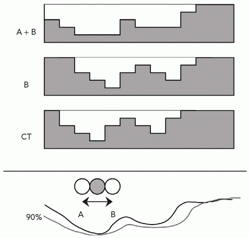 Figure 8A.7 Consider the range-compensator CT (bottom) designed given the static patient geometry represented by the planning computed tomography (CT) scan. In that scan, a “circular” inhomogeneous feature determined the thinnest part of the range-compensator. In the course of treatment, this feature can assume any position between the limits A and B. If the feature is at B, the range-compensator B (middle) would be most appropriate. In effect, one wishes the range-compensator, at any given point, to move with the features that affect its range shifting profile. This can be accomplished, at least for one feature, by selecting the thinnest part of the range-compensator profile within the smearing distance at every point. The resulting range-compensator A + B shows a significantly altered profile (top), which assures target volume coverage irrespective of the position of the offending feature but with a degradation of distal target volume conformality as indicated by the (hypothetical) 90% isodose line for the CT range-compensator (black line) compared to the 90% isodose line (gray line) of the A + B range-compensator. |
This approach is adopted in Figure 8A.8C and assumes, for our phantom, no range uncertainty so distal coverage is very tight. To ensure target coverage for up to 10 mm of lateral motion, the range-compensator designed in Figure 8A.8C is smeared by 10 mm and the aperture expanded by 10 mm, which results in the dose distribution in Figure 8A.8D. The dose overshoot near the lateral CTV edges is necessary to ensure CTV coverage given the CTV motion. It is clear that the high-dose region, which ensures target coverage under motion (Fig. 8A.8E), does not conform to the PTV. Moreover, a PTV designed to meet the dose requirements for the CTV for this anterior field would not equal the PTV designed to meet the same dose requirements for the same CTV for another field from a different approach. A PTV is unnecessary to determine the dose distribution ensuring target coverage under motion (Fig. 8A.8D) as the correct aperture size can be directly
derived from the CTV plus a margin for lateral motion (either breathing or setup errors). Figure 8A.8 proves, for charged particles, the inadequacy of the PTV for field design and the inadequacy in representing dose. For the latter, the PTV does not serve as an entity to specify the dose or as an entity to report the dose.
derived from the CTV plus a margin for lateral motion (either breathing or setup errors). Figure 8A.8 proves, for charged particles, the inadequacy of the PTV for field design and the inadequacy in representing dose. For the latter, the PTV does not serve as an entity to specify the dose or as an entity to report the dose.
 Figure 8A.8 Tumor in lung phantom. Gray and white areas are unit-density and lung density, respectively. The filled circle indicates the 50-mm diameter GTV. Also shown are the 60-mm diameter clinical target volume (CTV) (solid circle) and 80-mm diameter PTV (dashed circle). Isodose lines displayed are 50, 80, 95 (thick), and 100%. A: A plan designed to conform to the PTV with the tumor in its representative position. B: Same plan as (A) but for a 10-mm shift of the CTV. C: Plan conforming tightly to the CTV in its representative position. D: Same as (C) but with the aperture expanded by 10 mm and the range-compensator smeared by 10 mm. E: Same as (D) but for a 10-mm shift of the CTV. (Figure adapted from Engelsman M, Kooy HM. Target volume dose considerations in proton beam treatment planning for lung tumors. Med Phys. 2005;32:3549-3557.)4 |
One solution is to use different stages of the treatment planning cycle for reporting dose to the CTV and to critical structures. For this we propose the use of the terms initial beam, indicating the beam designed to tightly cover the CTV (i.e., Fig. 8A.8C), and final beam, indicating the beam altered to take into account uncertainties (i.e., Fig. 8A.8D). Dose to the CTV should be reported only for the initial beams as this is the dose distribution guaranteed to be delivered to the CTV. Dose to normal tissues on the other hand, should be reported using final beams as that is how the patient is actually treated. It is best, however, to actually simulate setup errors in the treatment planning system by using “final” beams and applying multiple shifts to the isocenter of the treatment plan, a method proposed by A. Lomax.
The tumor in lung phantom as shown in Figure 8A.8 was chosen because it maximizes the effects of density changes on the proton dose distribution. The resulting conclusions regarding the usefulness of the PTV do, however, apply in general, albeit with less dramatic consequences.
Dose Properties
As stated in the preceding text, the lateral penumbra is governed by the source size and the proton scatter in the patient and in the range-compensator. The source of the proton beam is not a physical point in the nozzle. Instead, it is a source produced by the many scatterers in the nozzle and has properties analogous to the source properties observed in electron fields. The source position and properties are reconstructed from the divergence and penumbral spreads observed in air. The latter are affected by the amount of material in the nozzle, most notably the range-modulation system and scatterers, which cause the proton beam to significantly broaden from the initial pencil beam size upon entry to the nozzle. The apparent source size of a double-scattered proton beam is in the order of 5 cm full-width at half-maximum. This is to be compared to the typical source size of 0.2 cm in a photon field. The effect of this large source size on the in-patient lateral penumbra can only be mitigated by, first, using a large source to axis distance and, second, by using a collimating aperture and place it as close as possible to the patient. The source to axis distance in a proton gantry is on the order of 300 cm and can be as large as 500 cm for a fixed beam line. The aperture is typically placed with a gap of 3 to 10 cm to the patient’s skin. This close proximity effectively reduces the source size by this gap over the source-to-axis distance (SAD), that is, by a factor of 50 to 100. This requirement to reduce the source size by placing the aperture close to the patient, coupled with the need of stopping the proton beam, results in considerable bulk for a proton multileaf collimators. Such multileaf collimators for double-scattered SOBP fields are not practical, perhaps even impossible, because of the needed bulk. In addition, the continuous exposure of the multileaf collimator to
proton radiation in close proximity to the patient will result in activation of the collimator and unwanted dose to the patient. Such multileaf collimators do become practical in other beam configurations and specifically those used in scanned proton beams.
proton radiation in close proximity to the patient will result in activation of the collimator and unwanted dose to the patient. Such multileaf collimators do become practical in other beam configurations and specifically those used in scanned proton beams.
The second contribution to the lateral penumbra is the scatter of the proton beam in the range-compensator and the patient. The scatter in the range-compensator is considered separately as it is a device external to the patient. The scatter from the range-compensator at a point in the patient is assumed, typically, to be due to the thickness of the range-compensator traversed by the ray from the source to the point of interest. That is, thick parts of the range-compensator will induce more scatter compared to thin parts which, in turn, will lead to cold and hot dose spots in the patient for irregularly shaped range-compensator. Such effects, therefore, can only be accurately modeled by treatment planning dose calculation models6 or Monte Carlo calculations.7
The final contribution to the lateral penumbra is scatter of the proton beam in the patient itself. The latter is, of course, unavoidable even if the contributions mentioned earlier are minimized. The in-patient scatter increases as a function of range, that is, penetration in the patient. This is in contrast to a photon beam penumbra which, to first order, is largely independent of depth as its major source is the creation and diffusion and disequilibrium of secondary electrons at the field edge. Therefore, the penumbra of a single proton field, although considerably sharper for shallow ranges compared to a single photon field, steadily increases and is comparable to a photon field at approximately 16 cm range and worse for higher ranges. The penumbra of a proton field, however, due to the continued forward direction of scattered protons in contrast to the laterally diffusing electrons, does not increase in low-density tissue. In lung tissue, for example, the penumbra of a photon field effectively triples whereas the penumbra of a proton field is unaffected.
The scattering and subsequent broadening of the initially, as it enters the nozzle, narrow and focused proton beam allows for a computational description of the proton field as a composite set of pencil beams. Each pencil beam is assumed to emanate from the source and have a lateral intensity (fluence) distribution described by a Gaussian distribution, that is, its lateral extent is characterized solely by the Gaussian spread, σ. The use of such a pencil beam formalism in proton dose calculation is quite accurate when compared to Monte Carlo except in those clinical situations with very high-density inhomogeneities as often are found in postsurgical patients with inserted stabilization hardware. The contributions to proton scatter, described in the preceding text, add individually to the Gaussian spread σ. Because of the Gaussian description, each individual contribution can be computed separately and added in quadrature with the other contributions to yield the total spread σ. The pencil beam formalism, albeit for electrons or protons, gives the dose to a point in the patient from a single pencil beam simply in terms of the lateral displacement of the point to the pencil beam and the fluence (i.e., number of particles per area) and the spread of the pencil beam at the depth of the point. The total dose to the point is then the sum of contributions from all pencil beams in the field.
As a representation of a physical phenomenon, the Gaussian description of a proton field as a set of proton pencil beams is more physically apt compared to the similar description for electron fields.8 For a proton pencil beam, the initial pencil beam retains its “identity,” that is, a proton initially contained within a given pencil beam retains its membership as the proton scatters little beyond the pencil beam direction and continues to travel along the direction of the pencil beam ray. The statistical description of scatter and the physical transport of the pencil beam are therefore correlated. For an electron pencil beam, however, the description at any given depth is statistical and describes the composite property of the set of electrons that appear at that depth. Both descriptions, to be sure, are valid in so far that each permits a characterization of the beam and dose produced in the medium. The close correlation between the physical and statistical description of the proton pencil beam permits the use of the pencil beam formalism for intensity-modulated proton fields as these are truly narrow beams of proton “pencils.”
The comparison stated in the preceding text of lateral penumbra to a photon field is for a single field irradiation. Single field irradiation is practical for proton fields as each field, alone, can deliver homogeneous dose to the target volume with sharp lateral and distal target conformation. Single field irradiation is not possible for photon fields, however, as a single field has no dose conforming properties of significance. The practice is therefore to always use a combination of fields, with IMRT being the most sophisticated form of combining fields and intensities. The effective penumbra in a treatment plan is thereby primarily formed by the combined intersections of the number of fields used in delivery. Figure 8A.9 shows the effect of the effective penumbra for a 50-mm cylindrical target centered in a 200-mm cylindrical phantom irradiated by rotating fields of protons and photons, both assumed to have zero, that is, infinitely sharp, lateral penumbra. The final effective penumbra, as measured as the distance between the 20% to 80% falloff, is 57 mm for the photon field and 12 mm for the proton field. Therefore, the intrinsic penumbra is largely insignificant, especially for the photon field. The difference in effective penumbra is caused by the full penetration of the photon beam compared to the zero dose beyond the distal falloff of the proton beam.
In clinical practice, an IMRT field is able to use the intrinsic penumbra of the photon field by judiciously choosing the field arrangements and dose constraints. This allows the intrinsic penumbra to be “fixed” along one surface, with a correlated effect of worsening the effective penumbra elsewhere. A classic example of this choice is the use
of IMRT in prostate treatments to achieve a sharp dose gradient between the prostate target volume and the abutting anterior rectal wall. In that situation, the “true” single field photon penumbra is realized. Current standard for proton prostate treatment (cf. Fig. 8A.11) is the use of right and left lateral fields with ranges on the order of 25 cm. A field of such a large range has a larger penumbra compared to a penumbra of an IMRT field. Obviously, the effectiveness of a treatment, especially if compared to another modality, depends on many physical and clinical factors and the intent here is to demonstrate a physical difference that must be considered, and modeled correctly in the treatment plan, to achieve the desired treatment objective.
of IMRT in prostate treatments to achieve a sharp dose gradient between the prostate target volume and the abutting anterior rectal wall. In that situation, the “true” single field photon penumbra is realized. Current standard for proton prostate treatment (cf. Fig. 8A.11) is the use of right and left lateral fields with ranges on the order of 25 cm. A field of such a large range has a larger penumbra compared to a penumbra of an IMRT field. Obviously, the effectiveness of a treatment, especially if compared to another modality, depends on many physical and clinical factors and the intent here is to demonstrate a physical difference that must be considered, and modeled correctly in the treatment plan, to achieve the desired treatment objective.
 Figure 8A.9 Consider a cylindrical phantom of 200-mm diameter with a centered cylindrical target of 50 mm. The target is irradiated with a 6-MV photon distribution (ignoring build-up dose) and a spread-out Bragg peak (SOBP) of range 125 mm and modulation 50 mm (C); both distributions have a field width of 50 mm, covering the width of the target, and an infinitely steep lateral falloff, that is, zero penumbra. The SOBP field dose plateau is centered on the target and covers it in depth. The fields are rotated 360 degrees around the target and yield the dose distributions shown in A and B. The left figure is an isodose contour plot (with fractional dose values) with the left half that from the SOBP field rotation and the right half from the 6- MV field. The figure (B) shows the cross-profile through the center of rotation and shows in the legend the effective penumbral falloffs, 12 mm for the SOBP and 57 mm for the 6 MV, as measured between the 20 and 80 dose values (indicated by the gray horizontal lines). |
Proton fields have the additional degree of freedom to achieve sharp dose gradients at multiple locations throughout the treatment volume. The most effective method to create such sharp dose gradients is through the use of intensity-modulated proton fields and analogous to IMRT. Proton fields, however, can also achieve multiple dose gradients through the use of patched fields. Patching for proton fields is the three-dimensional extension of matching the lateral edges of photon, and proton, fields. Patching can be achieved with proton fields for two reasons. First, a proton field can deliver homogeneous dose to the target volume with a single field. Therefore, target volume coverage can be achieved with multiple fields, each of which delivers homogeneous dose to at least one part of the target volume. Second, the sharp distal falloff of a proton field can be matched to another edge. In patching, the distal edge of one proton field is brought to the lateral edge of another proton field to achieve a continuous, near-uniform dose across the match (patch) surface. Figure 8A.10 illustrates the patch-field geometry and the field and target segmentations and patch steps necessary to achieve a patched field combination. The clinical example in Figure 8A.10 uses a set of three fields to achieve a sharp penumbra around the optic chiasm which is surrounded by a target volume. In a set of patch fields, one field is considered the “THROUGH” field and is the field which achieves typically the most target volume coverage. Any part of the target volume not treated by the THROUGH field, defined as that part of the target volume that is outside the 50% lateral dose edge of the through field, is treated by a patch field whose distal falloff is patched to the 50% lateral edge of the THROUGH field. This patching can be repeated until all segments of the target volume are covered.
The computation of patch field requires the computation of the intersection surface of the 50% lateral THROUGH field edge and the design of the range-compensator of the patch field such that the distal 50% falloff matches the THROUGH field 50% surface. This computation, of course, requires treatment planning software. In addition, the above-mentioned uncertainties in the position of the distal falloff require special consideration. In practice, the patch field edges are feathered over the target volume to mitigate uncertainties in dose across the patch field edges. Such feathering is, in our practice, achieved by alternating the choice of THROUGH and patch field precedence as such fields typically are paired (in contrast to the example in Figure 8A.10 where one THROUGH and two patch fields were used). It is not possible to feather the THROUGH field lateral edge, as it is determined and fixed by virtue of the aperture edge. It is possible to “modulate” the distal falloff position by choosing a mixture of ranges for the patch field. Such a mixture of ranges will “dull” the distal falloff and hence could reduce the effect of the distal range uncertainty. This mixing is not typically used in clinical practice due to the overhead of the increased number, one per range, of deliverable fields required.
The computation of patch field requires the computation of the intersection surface of the 50% lateral THROUGH field edge and the design of the range-compensator of the patch field such that the distal 50% falloff matches the THROUGH field 50% surface. This computation, of course, requires treatment planning software. In addition, the above-mentioned uncertainties in the position of the distal falloff require special consideration. In practice, the patch field edges are feathered over the target volume to mitigate uncertainties in dose across the patch field edges. Such feathering is, in our practice, achieved by alternating the choice of THROUGH and patch field precedence as such fields typically are paired (in contrast to the example in Figure 8A.10 where one THROUGH and two patch fields were used). It is not possible to feather the THROUGH field lateral edge, as it is determined and fixed by virtue of the aperture edge. It is possible to “modulate” the distal falloff position by choosing a mixture of ranges for the patch field. Such a mixture of ranges will “dull” the distal falloff and hence could reduce the effect of the distal range uncertainty. This mixing is not typically used in clinical practice due to the overhead of the increased number, one per range, of deliverable fields required.
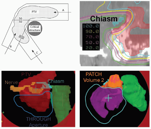 Figure 8A.10 The top right figure illustrates a target volume wrapped around a critical structure. A single field cannot cover the target volume because the use of the distal falloff is precluded to achieve the desired sharp dose gradient. A “THROUGH” field A is chosen to cover as much of the target volume as possible. Its range-compensator is designed to achieve a distal falloff that matches the distal target volume. The first patch field B is chosen to cover most of the target volume outside the 50% lateral falloff of field A. The field B range-compensator is designed such that the distal falloff matches the 50% lateral falloff of field A, thereby achieving 100% continuous dose across the patch surface. The procedure repeats with a patch field C to cover that target volume that is not covered by fields A and B. The bottom figures show the beam’s eye view for a through field (bottom-left) and the first patch (bottom-right), that is, the purple and orange volume is the PTV volume outside the through aperture. The orange volume in the bottom right figure is the volume that requires a third patch field as it is not covered by the aperture. These three fields were necessary to achieve a sharp dose gradient around the optic chiasm surrounded by target volume. The dose distribution in a coronal plane around the optic chiasm is shown in the top right figure. |
INTENSITY-MODULATED PROTON THERAPY
Intensity-modulated proton therapy (IMPT) offers improved conformality of proton dose distributions to the
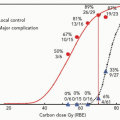
target volume and increased sparing of healthy tissue compared to both three-dimensional conformal proton therapy and photon IMRT. Proton IMPT treatments are routinely delivered at the Paul Scherrer Institute (PSI) in Switzerland.9,10 The experience at PSI demonstrates improved tissue sparing in a number of sites, including intracranial, nasopharyngeal and paraspinal lesions.9,11, 12, 13, 14 Intensity-modulated particle therapy with carbon ions was, until recently, routinely performed at the German Society for Heavy Ion Research (GSI, Darmstadt).15,16 This clinical practice will be resumed at the new ion-therapy facility currently (2006) under construction in Heidelberg, Germany.
target volume and increased sparing of healthy tissue compared to both three-dimensional conformal proton therapy and photon IMRT. Proton IMPT treatments are routinely delivered at the Paul Scherrer Institute (PSI) in Switzerland.9,10 The experience at PSI demonstrates improved tissue sparing in a number of sites, including intracranial, nasopharyngeal and paraspinal lesions.9,11, 12, 13, 14 Intensity-modulated particle therapy with carbon ions was, until recently, routinely performed at the German Society for Heavy Ion Research (GSI, Darmstadt).15,16 This clinical practice will be resumed at the new ion-therapy facility currently (2006) under construction in Heidelberg, Germany.
The term IMPT is used analogous to IMRT and is a specific delivery mode available with scanned proton beams. In general, scanned beams can be used to create arbitrary dose distributions. Unlike SOBP proton field treatments, in which each field delivers a uniform (within a few percent) dose to the whole target volume, or a subsection as in patch-field treatments, individual IMPT fields typically deliver nonuniform dose distributions (e.g., see Fig. 8A.11). Similar to IMRT with photons, these nonuniform field contributions combine to produce the desired therapeutic dose distribution, which may be sculpted according to the clinical prescription: Either to be uniform, as is commonly required in treatment protocols, or nonuniform (to deliver, e.g., a simultaneous dose boost to a subvolume within the target). An important difference from photon IMRT is that the pronounced Bragg peak of the proton depth-dose distribution introduces an additional degree of freedom in modulation of the dose in depth along the proton beam axis, as well as modulation of the intensity in the transverse plane available in IMRT and IMPT. To take full advantage of this possibility to sculpt the dose in depth, IMPT treatments use narrow proton pencil beams which can be magnetically moved over the transverse plane while changing energy and intensity to control the dose to a point.
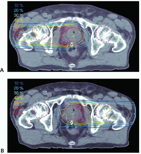 Figure 8A.11 Intensity-modulated particle therapy (IMPT) plan for a prostate patient: dose contributions delivered by (A) the right lateral and (B) left lateral fields add to the uniform dose prescription of 79.2 Gy (relative biological effectiveness [RBE]). Dashed purple lines designate the outlines of the prostate, planning target volume, rectum, bladder, and femoral heads. The isodose values are in percentage of prescription dose per field; the composite yields the desired 100% prescription dose to the target volume. Note, specifically, that each field is essentially a mirror image of its partner, and that the optimization resulted in a proximal high dose. (Patient data provided by Dr. W. U. Shipley.) |
The methods of intensity modulation, summarized by Lomax17 and illustrated in Figure 8A.12, demonstrate the flexibility of using scanned proton beams to create dose distributions in a medium. One method, dubbed “distal edge tracking” or DET, originally proposed by Deasy et al.,18 is to distribute pristine Bragg peaks of varying intensities near the distal surface of the tumor by setting the respective pencil beam energies to those of the radiologic depths to the distal surface. The “threedimension (3-D) modulation” method places Bragg peaks throughout the 3-D target volume. Such 3-D-modulated fields can be delivered by consecutively irradiating layers of equal radiologic depth within the target, using a single value of proton energy per layer while changing, again, the intensities of the pencil beams in the transverse plane (see Fig. 8A.13). Such use of multiple consecutive layers, each at constant radiologic depth, is dubbed “layer scanning.” An alternative is the “depth scanning,” a discrete irradiation mode in which, for each pencil beam position, a number of depths positions are irradiated consecutively, making the proton beam penetration depth the fastest varying scan coordinate. The adjustment of proton range in tissue is achieved with insertion of range compensating material, for example, Lucite plates or wedges, in the beam path.19 The 3-D-modulation method is the most general method of applying scanned beams and is, in general, synonymous with the term IMPT.
Spread-out Bragg peak modulation, as in scattered proton techniques, can also be applied by creating individual SOBP distributions for each pencil beam axis. This method is dubbed a “two-dimension (2-D) modulation” technique. In 2-D modulation, each pencil beam covers the target with an SOBP of constant modulation width but with individual, per pencil beam, intensities. It is essentially the DET method using a spread-out Bragg peak instead of a pristine Bragg peak. A further improvement in conformality, dubbed “2.5-D modulation,” is achieved if the modulation width of an individual pencil beam SOBPs is adjusted to equal the thickness of the target traversed by that pencil beam. Note that the SOBP dose modulation in 2-D and 2.5-D techniques, namely the approximately uniform-dose plateau along the pencil beam axis, does not strictly require
the use of a modulating device (e.g., a range-modulator wheel). The SOBPs can be delivered by depth scanning and delivered with the pristine proton beam, by changing the proton energy and intensities from layer to layer.
the use of a modulating device (e.g., a range-modulator wheel). The SOBPs can be delivered by depth scanning and delivered with the pristine proton beam, by changing the proton energy and intensities from layer to layer.
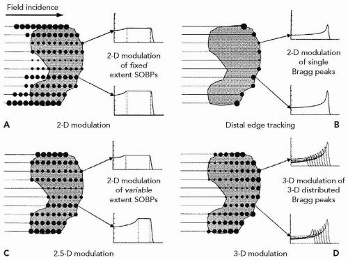 Figure 8A.12 Four approaches to proton intensity-modulated radiation therapy (IMRT). Positions of solid circles represent individual Bragg peak positions and circle diameters symbolize relative intensities. Note, however, that, for clarity, circle diameters represent variations in the free modulation parameters of each method only (see text). Any fixed modulation of Bragg peaks, for example, to form the spread-out Bragg peaks (SOBPs) in A and C, are not represented in these diagrams. Representative depth-dose curves for each method are indicated on the right hand side of each diagram. Note also that each diagram represents the free modulation of pencil beams from only one of potentially many field directions. (Reprinted with permission from Lomax A. Intensity modulation methods for proton radiotherapy. Phys Med Biol. 1999;44:185-205.) |
It is therefore important to note that the differences between the various delivery modes are not technologic. All methods use the same delivery system: a composite set of narrow proton pencil beams which vary in intensity and energy. The only differences are, first, in dosimetric abilities and, second, in robustness of delivered and desired dose in the presence of uncertainties. Figure 8A.14 illustrates some differences between 2.5-D and DET approaches in terms of robustness of dosimetric outcome of the plan to uncertainty in the proton range.
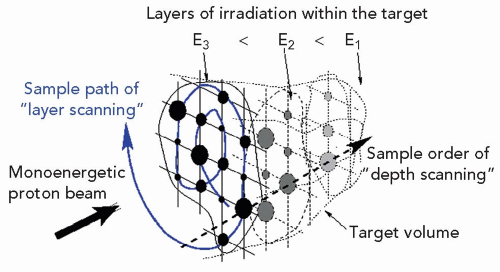 Figure 8A.13 An illustration of some of the basic concepts in the dynamic delivery of intensity-modulated particle therapy (IMPT). The target is irradiated in successive layers, each at a constant (radiologic) depth, indicated by the energies E1, E2, and E3. Each layer contains a set of pristine Bragg peaks of varying fluence to achieve the desired dose variation within the layer. The control sequence of irradiation within a layer, the “sample” path described by the sequence of central axes of the pristine pencil beams, can be arbitrary and is only limited by the control system. |
Field-specific range-compensators are strictly speaking not required for IMPT, as the Bragg peak “pull-back” can be achieved by an energy adjustment, but may be useful in certain scenarios. The spatial resolution of a compensator, typically 3 mm, compares favorably to the size of pencil beams available for IMPT treatments, with full widths at half-maximum of 10 mm and higher. These pencil beam widths are primarily controlled by the beam line magnets but are adversely affected by the traversal of the proton beam through materials to reach the patient. The high lateral resolution of the range-compensator, combined with a depth resolution of better than 1 mm, may allow for better conformality to the distal target surface than can be achieved with the energy modulation alone. In IMPT, using the 3-D modulation method, the number of required irradiation layers may be reduced with the use of compensators, as illustrated in Figure 8A.15. While IMPT-capable treatment planning systems, such as KonRad20,21 and VoxelPlan,22 support all or most of the modulation methods listed in the preceding text, with or without the use of range-shifting devices, to date, most publications on plan comparisons or clinical reports used the 2.5-D and 3-D modulation methods without range-compensators.
Related posts:

Stay updated, free articles. Join our Telegram channel

Full access? Get Clinical Tree


