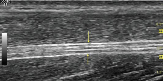
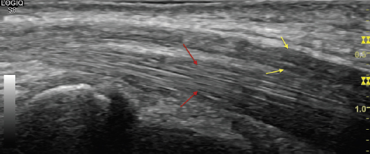
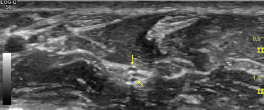
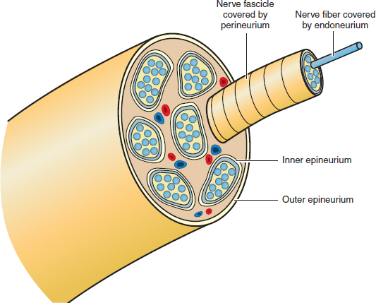
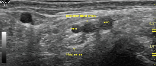
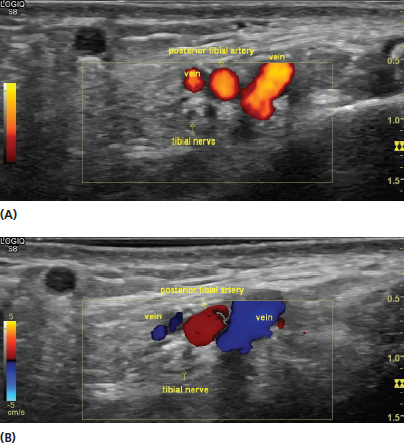
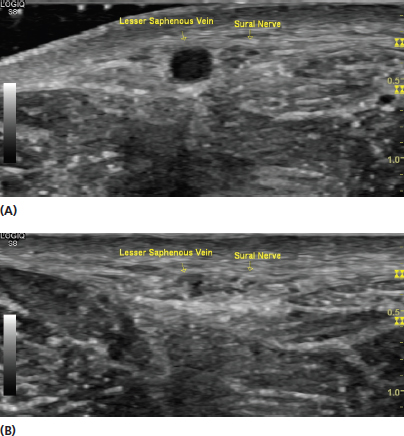
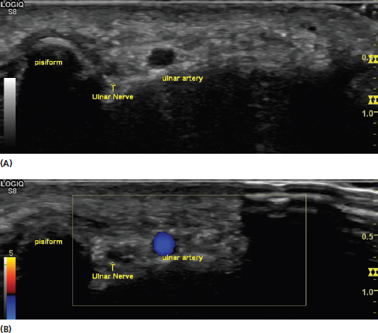
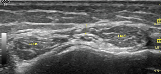
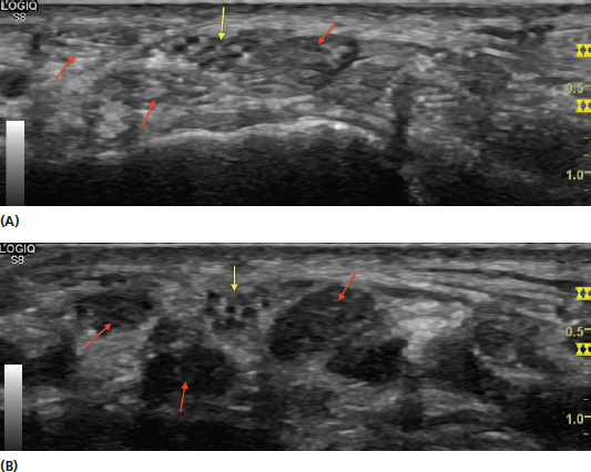
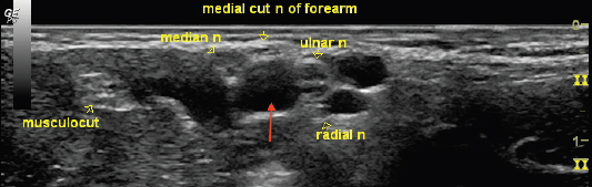
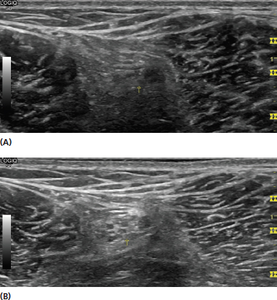
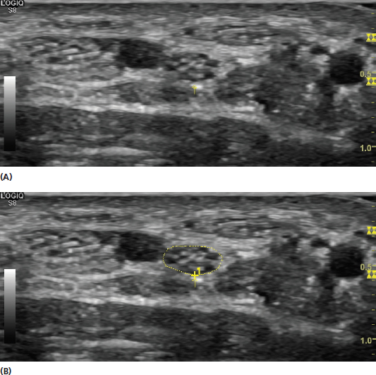
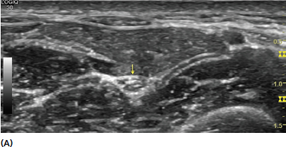
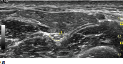
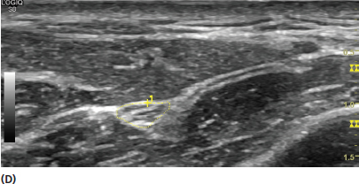
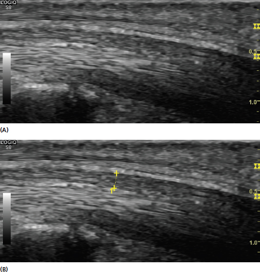
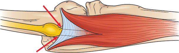
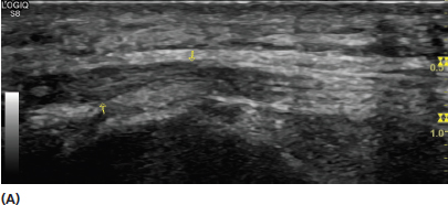
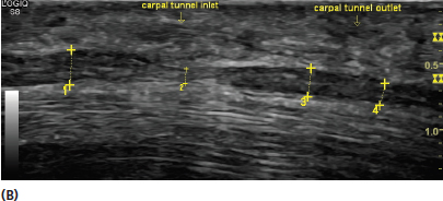
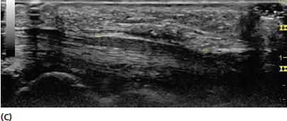
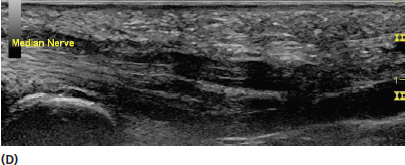
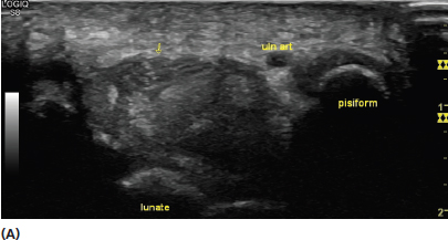
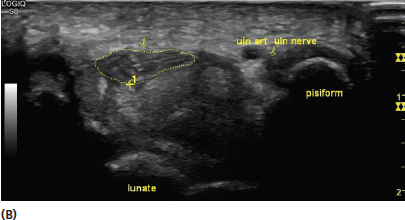
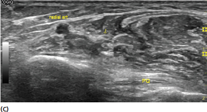
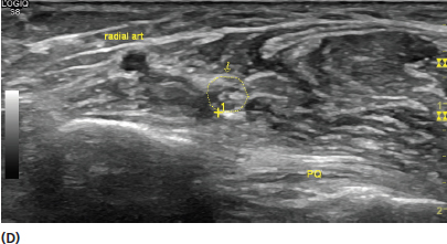
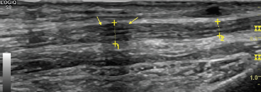
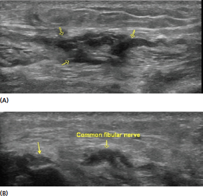
The appearance of nerve on ultrasound is that of an uninterrupted fascicular pattern (Figure 9.1). This differs from the intercalated pattern typical of tendons (Figure 9.2). The hypoechoic (dark) nerve fascicles are seen among the hyperechoic (bright) epineurium. In short-axis view, this creates an appearance that is frequently described as resembling a “honeycomb” (Figure 9.3).

Histologically, the fascicles are enveloped by perineurium and the nerve fibers are covered by endoneurium (Figure 9.4). The outer sheath is termed the epineurium or “outer epineurium” and the tissue between the fascicles and the outer epineurium is sometimes referred to as the “inner epineurium.”

Nerves often have arteries and veins that accompany them and it is necessary to recognize them for reliable identification (Figure 9.5). Doppler imaging can be used to attempt to see flow in suspected vessels (Figure 9.6). Veins can be identified by their compressibility (Figure 9.7). Nerves generally have intraneural vessels; however, these are usually not readily identifiable on ultrasound. It is important to reliably identify the larger vascular structures so that they are distinguished from the nerve when performing measurements. Often, scanning proximally and distally can improve this determination. Use of Doppler is also helpful when needed (Figure 9.8).

Nerves are generally easier to identify in short-axis view. Efforts should be made to identify the fascicular architecture and distinguish it from the surrounding tissue (Figure 9.9). Scanning back and forth can help distinguish the nerve tissue from other surrounding tissue. Other techniques used to improve the conspicuity of the nerve include movement of the surrounding tissue, rocking or toggling the transducer, or moving to a position where there is more contrast from the surrounding tissue relative to the nerve (Figure 9.10). Using conspicuous anatomic landmarks can help identify the location of more challenging nerves (Figure 9.11). When following the course of a nerve in short axis, it is often more effective to scan rapidly rather than too slowly to accentuate the contrast in tissue. Using liberal amounts of coupling gel is helpful to facilitate that.

The examiner should be vigilant about the amount of pressure that is being placed on the tissue by the transducer. Excessive pressure can alter the shape of the underlying nerve as well as compress the surrounding tissue. This includes surrounding vascular structures such as veins that can often help with localization (Figure 9.7). In some circumstances, the use of higher transducer pressure can improve the image quality of a relatively deep nerve (Figure 9.12).

FIGURE 9.12 Sonograms of short-axis views of the same sciatic nerve (yellow arrows) demonstrating the potential benefit of increased transducer pressure. The image in (A) is with light transducer pressure and the image in (B) has increased transducer pressure. Note the increased resolution of the fascicular architecture of the deep sciatic nerve with the increased transducer pressure (B).

Nerves can also be precisely measured with most ultrasound instruments. Cross-sectional area measurements of nerves in short axis are the most commonly used. This can be performed both by direct tracing inside the border of the nerve or more indirectly by the use of calipers and an ellipse. With either technique, the measurement should be performed on the inner aspect of the outer epineurium (Figure 9.13). Once adequate experience has been gained, the direct tracing method is generally preferable for reliability. Care should be used to establish that the measurement of the nerve is being obtained with the image as perpendicular as possible to obtain a reliable measurement. This usually means that the transducer should be oriented to create the smallest cross-sectional area possible while maintaining a short-axis plain. Obliquity of the image can create an artifactually inaccurate large cross-sectional area (Figure 9.14). With nerves that are relatively small in size, measurement of the diameter in short axis rather than cross-sectional area is more practical because reliable cross-sectional area cannot be obtained.

FIGURE 9.13 Sonograms of short-axis views of a nerve. The image in (A) is the nerve with the transducer place in perpendicular position noted by the smallest cross-sectional area. The image in (B) is the same picture with the nerve measured using the direct tracing method. Note that the trace is at the inner border of the outer epineurium.

The diameter is also used for measurement of nerves in long-axis view (Figure 9.15). Measurement in this plane is often more challenging because the nerves often do not follow a straight course. The nerve should be scanned sufficiently to establish that the transducer is appropriately aligned over the maximum diameter of the nerve. The surrounding region should be assessed to reliably confirm that only nerve tissue is being measured. The diameter measurements should also be correlated with those obtained in short-axis view to confirm accuracy.

FIGURE 9.15 Sonograms of a long-axis view of the median nerve (A) as well as a view of the same image with diameter measurement (B).

NERVE PATHOLOGY

The appearance of peripheral nerves on ultrasound due to focal injury or generalized disease can be variable and is often related to the extent of the pathology. Focal neuropathies often present with abnormal swelling that is usually just proximal to the site of the injury (Figure 9.16). However, there can be some variation in the presentation (Figure 9.17). Precise measurements and use of side-to-side comparisons when appropriate can be helpful. The measurements most frequently used are in short axis but long-axis views also provide needed perspective. At the current time, there is considerable variation between published normal values with respect to cross-sectional areas with many peripheral nerves. This seems to reflect variation in the manner in which the nerves are measured, among other factors. The median nerve at the carpal tunnel has been the most frequently studied nerve with ultrasound. Many studies of the median nerve have established slightly different normal values, but there is general consensus that a cross-sectional area of greater than 13 mm² is highly predictive for the presence of median neuropathy at the carpal tunnel. Many feel that a cross-sectional area in the realm of 10 to 13 mm² is also abnormal. Ultrasound also has sensitivity for identifying median neuropathy that is relatively similar to electrodiagnostic studies. Ultrasound, to this point, has not been shown to be as valuable as electrodiagnosis for determining the relative severity of neuropathies.

FIGURE 9.16 Illustration of a nerve entrapment. The nerve shows focal enlargement just proximal to the entrapment site (red arrows).

Peripheral nerve size has variation with body mass index, gender, age, and other factors. Using unaffected areas of a peripheral nerve for reference can be helpful in determining pathology (Figure 9.18).

In addition to size measurement, identification of changes in the normal architecture of the nerve can also reveal neuropathy (Figure 9.19). There is no consistently good correlation between the size of nerves and relative severity of the neuropathy, but visual disruption of the normal fascicular architecture is more often associated with axonal injury. Complete transection of the nerve (neurotmesis) can typically be distinguished from a nonfunctional nerve with the connective tissue intact (complete axonotmesis) on ultrasound (Figure 9.20). This is an advantage of ultrasound over routine physical examination and electrophysiologic studies, which cannot reliably distinguish these conditions. This determination can enhance acumen for treatment decisions, including surgical intervention.

FIGURE 9.17 Sonograms demonstrating long-axis views of nerve swelling in different entrapment neuropathies. The image in (A) shows a typical entrapment pattern with an ulnar neuropathy at the elbow with distal constriction (superior yellow arrow to the right) and a more proximal focal enlargement (inferior yellow arrow to the left). The other images show postoperative median neuropathy at the carpal tunnel. In (B), there is focal constriction from scarring in the middle and enlargement both proximally and distally to that level. The image in (C) shows a diffuse enlargement in between two areas of focal constriction. In (D), the median nerve is diffusely swollen with multiple areas of tethering from scar. These images demonstrate examples of different presentations of focal neuropathies and reflect the need to examine the entire area of potential pathology.

Ultrasound can also identify factors that can be the source of peripheral nerve injuries. This includes intrinsic and extrinsic tumors, abnormal movement and subluxations, encroaching tissue, hematoma, scar and other postsurgical changes, as well as foreign bodies. In addition increased vascularity can be seen in some peripheral nerve lesions with Doppler imaging. Ultrasound is a valuable tool for assessment of peripheral nerves in a vast array of predisposing conditions. As with other tissues inspected in a musculoskeletal or neuromuscular evaluation, pathologic findings should always be considered within the appropriate clinical context, including the information derived from the history and physical examination.

Related posts:

Foreign Bodies Image Optimization Scanning Techniques and Ergonomics Physics of Ultrasound Ultrasound Guidance for Injections Imaging Tendon

Stay updated, free articles. Join our Telegram channel

Join