Georgeta Mihai, PhD
This chapter is intended to give the reader a basic introduction to the physical principles of cardiovascular magnetic resonance (CMR). The essential physics of signal generation and image formation are briefly reviewed, and the pulse sequences and techniques used for each of the major functional categories of CMR are discussed in moderate detail. For more in-depth coverage of these topics, please refer to publications cited in references 1–4.
THE ESSENTIAL PHYSICS
THE RESONANCE PHENOMENON
Magnetic resonance imaging (MRI) relies on the nuclear magnetic resonance (NMR) phenomenon—a characteristic of atomic nuclei which possess an odd total number of protons and neutrons. Each of these nuclei exhibits a net spin angular momentum and an associated magnetic moment. The ratio between the angular momentum and the magnetic moment is a constant known as the gyromagnetic ratio (λ), which is specific to the particular magnetically active nuclei. Resonance refers to the phenomenon by which the above-specified nuclei selectively absorb and later release radiofrequency (RF) energy that is unique to the element and its chemical environment. This resonance is the source of signal used in MRI; it is a signal emitted by the molecules of the body after RF energy is applied to the tissue.
There are a few biologically significant elements that have the required odd number of nucleons: 1H, 17O, 19F, 23Na, and 31P. Based on its magnetic moment strength, isotopic abundance, and biological concentration, the hydrogen (1H) nucleus is the basis for nearly all clinical MR imaging. While each hydrogen proton has a very small magnetic moment, the additive effect of many individual protons (about 6.6 × 10²² hydrogen nuclei per gram of water) gives rise to a detectable net magnetic moment when the tissue sample is placed in a strong magnetic field. The main static magnetic field (B0) generated by a clinical MRI system is typically between 0.2 tesla (T) and 3.0 T, or roughly 30,000 times larger than the earth’s magnetic field—approximately 50 micro tesla (μT). The magnetic moment vectors of protons when subjected to such a strong external magnetic field will align themselves either parallel (lower energy state) or antiparallel (higher energy state) with the direction of B0. A small majority of spins (hydrogen nuclei) will come to equilibrium in the lower energy state parallel to B0 giving rise to the net magnetic moment—the origin of the MRI signal (Figure 1-1). In addition, when exposed to an external magnetic field, the protons exhibit precessional motion, similar to a spinning toy top that precesses about the earth’s gravitational field. The protons precess around B0 with a frequency that is directly proportional to B0 by the element specific constant of proportionality, the gyromagnetic ratio. This precessional frequency, ωL, known as the Larmor frequency is defined by Equation 1-1, the Larmor equation:
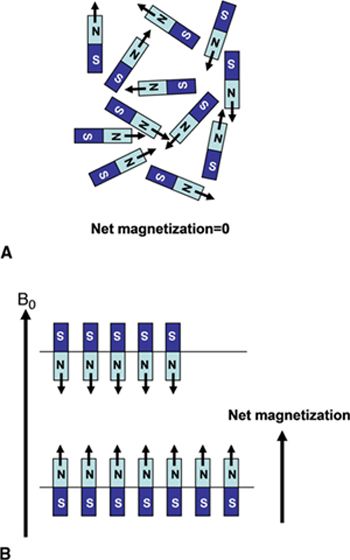
FIGURE 1-1 (A) Normal, random orientation of the individual 1H spins results in zero net magnetization. (B) The application of a strong magnetic field, B0, forces the spins to align either in a parallel or antiparallel direction with the applied field. A slight excess number of spins tends to align in the low energy state parallel with B0 and results in a net magnetization. (Reprinted with permission from Wiley-Blackwell from Principles and Practice of Cardiac Magnetic Resonance in Congenital Heart Disease: Form, Function and Flow.)
![]()
The resonance phenomenon takes place when a pulsed RF field, B1, with amplitude on the order of micro tesla and duration on the order of milliseconds, is applied with an oscillation frequency that matches the Larmor precessional frequency of the nuclear magnetization. During the application of RF energy, ie, RF excitation, the additional precession about the B1 field brings the spins into phase coherence and causes the net magnetization vector (M) to rotate away from alignment with B0. The angle of deflection of the net magnetization from the B0 axis is called flip angle and is proportional to the amplitude and duration of the RF pulse. A 90-degree RF pulse will rotate the entire net magnetization from the longitudinal axis (B0 or z-axis, by convention) into the transverse or x–y plane to create transverse magnetization Mxy. Any flip angle that is not an integer multiple of 0 or 180 degrees will result in some transverse component of magnetization. It is only this transverse component that is detectable by the receiver coils used in MRI; hence RF pulses that create transverse magnetization are often referred to as excitation pulses. Over time, the net magnetization of the hydrogen nuclei tends to align itself back along the longitudinal axis, as this is the lowest energy state. Excitation pulse flip angles of less than 90 degrees leave some longitudinal magnetization aligned with the external magnetic field, and thus can be more rapidly tipped again into the transverse plane with maintained signal level. Thus, MRI involves the application of a series of pulses designed to repeatedly tip the net longitudinal magnetization into the transverse plane where the MR signal can be detected.
MRI RELAXATION TIMES
Following the application of an RF excitation pulse, 2 concurrent events occur:
(1) The magnetic axes of the protons immediately begin to realign themselves with the B0 field (along the longitudinal or z-axis) with a time constant (T1) called the longitudinal or spin-lattice relaxation time. This relaxation occurs as RF energy is released back into the environment/lattice as the spins fall back into the lower energy equilibrium state.
(2) Transverse magnetization, Mxy, begins to decay with a time constant (T2) called the transverse or spin-spin relaxation time. The decay of transverse magnetization is due to the loss of phase coherence caused by random spin-spin interactions. As a spin is exposed to the magnetic moments of neighboring spins, its precessional frequency will change in relation to the variations in the local magnetic field according to the Larmor equation (Equation 1-1); different spins will experience different magnetic fields and will therefore precess at slightly different frequencies. As the spins precess at different frequencies, over time they fall out of synchrony with each other and are said to lose phase coherence. As a result, the net transverse magnetization begins to decay.
The Mxy component of the net magnetization precessing about the B0 field induces a time-decaying oscillating voltage (free induction decay signal—FID) into an RF antenna (receiver coil) positioned perpendicularly to the x–y plane (Figure 1-2); this is the source of the magnetic resonance signal used in MRI. Dynamic spin-spin interactions as well as static magnetic field inhomogeneities (magnetic field imperfections and/or magnetic field susceptibility differences between adjacent tissues) contribute to the decay of Mxy. The time constant that characterizes this combined process is called T2*, whereas T2 only includes the effects of random spin-spin interactions. The transverse magnetization dissipates long before recovery of longitudinal magnetization, and as such T1>T2>T2*. These relaxation parameters as well as the spin (proton) density (PD—number of spins per unit tissue volume) are fundamental, intrinsic properties that are exploited by MR imaging to differentiate and characterize tissues.
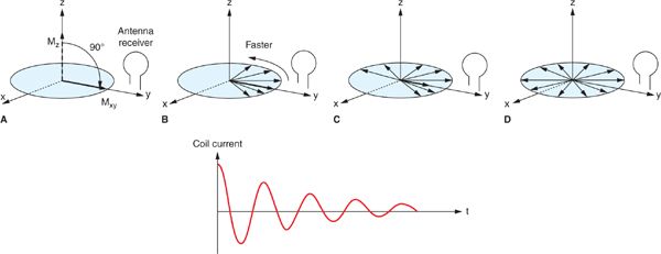
FIGURE 1-2 Conversion of a longitudinal magnetization, Mz into transverse magnetization Mxy by a 90-degree RF pulse, results in an initial pulse coherence of the spins causing a maximum current in the antenna receiver (A). As individual spins start de-phasing (B, C, D), both Mxy and the oscillating current decrease in time to zero. (Reprinted with permission from Wiley-Blackwell from Principles and Practice of Cardiac Magnetic Resonance in Congenital Heart Disease: Form, Function and Flow.)
IMAGE FORMATION
A detailed description of the process by which image information is encoded into the MRI signal is beyond the scope of this chapter. A basic understanding can be formed, however, from the fundamental principle of the Larmor equation (Equation 1-1) that linearly relates precessional frequency to the magnetic field strength. In an MRI system, additional gradient coils are built into the bore to generate linear, controlled variations of the B0 strength in x, y, and z directions. These linear changes in B0 translate into linear changes in the Larmor frequency as a function of position. Thus, spatial localization of the MR signal is made possible by varying the frequency and phase of the magnetization as a function of position. The image encoding process, while somewhat different for the through-plane (slice selection) and in-plane (frequency-encoding and phase-encoding) directions, is entirely based on the control of resonant frequency as a function of position via the gradient coils (Figure 1-3). By temporally varying the gradients, the frequency and phase of the spins’ precession become time and location dependent. In this manner the MR signals received from different locations can be distinguished from one another and the MR image can be formed.
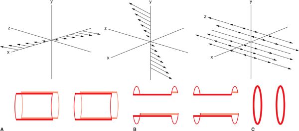
FIGURE 1-3 Diagram showing the field gradients (top) and saddle gradient coil (bottom) for the x (A), y (B), and z (C) Cartesian directions in a magnet bore. Magnetic field gradients of any arbitrary orientation can be generated by simultaneous activation of the different gradient coils. (Reprinted with permission from Wiley-Blackwell from Principles and Practice of Cardiac Magnetic Resonance in Congenital Heart Disease: Form, Function and Flow.)
Slice selection, that is the RF excitation of a single, thin slice, or slab of tissue which in turn provides the signal for an individual image, is achieved by turning on a gradient while a band-limited RF excitation pulse is applied. The slice select gradient creates a linear distribution of precessional frequencies along its direction; by matching the frequency content (ie, center frequency and bandwidth) of the RF pulse with the resonant frequencies of the spins in the desired slice, only those spins precessing in the range of frequencies contained within the RF pulse will be tipped into the transverse plane. Thus, the MR signal will emanate from a single, thin slice of tissue. Any arbitrary slice plane can be selected by combining gradients in x, y, and z directions. Following slice selection, the steps of phase and frequency encoding are used to encode the spatial frequency content of the image into the acquired MR signal.
k-SPACE
In order to discuss the processes of frequency and phase encoding used to create a two-dimensional (2D) image from the excited slice, it is necessary first to gain a basic understanding of the concept of k-space. k-space is the complex, 2D matrix that represents the spatial frequency content of the image. The signals acquired in an MRI scan do not directly correspond to image space, but rather represent the spatial frequency or k-space content of the image. Each point in k-space represents an individual spatial frequency or sinusoidal variation in signal intensity across the image. According to the Fourier theory, any signal (which may be multidimensional, as in the case of 2D or 3D images) can be represented as the sum of individual sine waves of different frequencies. The conventional MRI encoding process encodes each received signal into a raster line of sampled points across k-space. The amplitude of each point in k-space represents the relative contribution of a single spatial frequency to the overall image content; thus each point in k-space contributes to the signal of all image pixels. Spatial frequencies can be thought of as representative of the rate of spatial variation in pixel intensity in the image. Stated in another way, low spatial frequencies near the origin or center of k-space correspond to gross image features and contrast, while high spatial frequencies located further from the k-space origin correspond to fine details and image resolution. The Fourier transform defines the relationship between spatial frequency (k-space) and image space and is used to calculate or “reconstruct” images from the k-space data. For a faithful representation of the imaged object, the entire range of high and low spatial frequencies contained in the image must be sampled. This concept links image resolution with scan time; more lines of data must be sampled to cover the outer reaches of k-space, and this sampling of additional lines takes extra time.
In most MRI techniques the k-space data matrix is filled by sampling equally spaced parallel lines along the kx direction; these are referred to as phase-encoded k-space lines. Each line of k-space data therefore corresponds to one specific spatial frequency in the phase encoded direction (ky), and contains all spatial frequencies in the frequency encoding direction (kx). This so-called Cartesian trajectory, since k-space is sampled on a Cartesian grid, is widely used in almost all magnetic resonance imaging applications, including CMR (Figure 1-4A). Other trajectories through k-space such as radial and spiral are possible, but these can be more sensitive to system imperfections and have not been widely used in clinical applications.
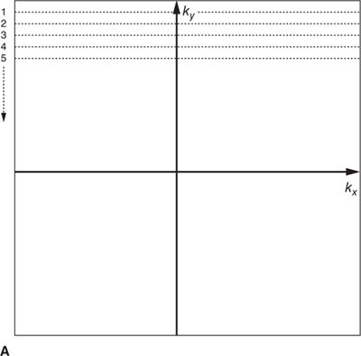
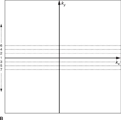
FIGURE 1-4 Cartesian k-space acquisition. (A) Standard or top-down k-space order (B) Centric k-space order
As mentioned previously, the outer k-space lines contain higher spatial frequencies representing information related to the finer details and image resolution. The order with which k-space lines are sampled can vary depending on the application. For example, in some contrast-enhanced angiography scans, the central region of k-space may be sampled first to capture the overall image contrast information while the arteries are filled with contrast agent, but before the contrast agent has reached the veins. This “centric” or “center-out” k-space trajectory starts at the center of k-space and works outward alternating sampling on positive and negative sides of the origin toward the edges of k-space (Figure 1-4 B).
PULSE SEQUENCES
The pulse sequence is a kind of recipe or program that prescribes the timing, order, polarity, amplitude, phase, and frequency of the RF pulses and gradients used to create MRI images. By varying the combinations of RF and gradient pulses, the number of possible pulse sequences is virtually endless. Echo time (TE), repetition time (TR), RF pulse combinations and flip angles, echo formation strategies, and preparatory pulses designed to enhance or suppress signals based on various MR properties can all be manipulated to control the sensitivity of the image appearance to a fantastic array of physiological parameters. Thus, the wide variety of pulse sequences is the source of MRI’s tremendous flexibility and also a major source of difficulty in understanding how MRI works. Nevertheless, the many pulse sequence types can be split into 2 main categories: (1) Spin echo; and (2) Gradient echo. While the MR signal could be sampled immediately after RF excitation, this would not permit time for the necessary gradient pulses used to encode spatial information into the signal. Instead, 2 basic strategies are used to form an “echo” of the MR signal sometime (TE) after the RF excitation pulse to allow time for spatial encoding and also to impart specific contrast weighting. In a typical spin-echo sequence, a 90-degree excitation RF pulse is followed by a refocusing 180-degree RF pulse that re-establishes phase coherence on the Mxy plane; this allows the formation of an “echo” that is encoded and sampled to fill 1 line of the k-space raw data matrix. In a spin-echo sequence, the echo amplitude is scaled by T2 signal decay; the static intrinsic B0 inhomogeneities and tissue susceptibility are corrected by the 180-degree refocusing pulse and echo formation, thereby avoiding sensitivity to T2*. In gradient-echo sequences, on the other hand, there is no refocusing RF pulse; the echo is formed by applying gradients with opposing polarity during signal acquisition. There is no correction of B0 field inhomogeneity and susceptibility in gradient-echo sequences and the echo amplitude is scaled by T2* effects rather than T2.
MR images generally display contrast that is based on T1, T2, T2*, or PD, or a combination of them, although flow and motion also play a major role in image contrast, particularly in cardiovascular imaging applications. The simplest method to control image contrast characteristics is by varying the TR and TE. The TR is the time between successive RF excitation pulses applied to the same slice, while TE is the time between the initial RF pulse and the center of the echo. The TE tends to be much longer for spin-echo than for gradient-echo sequences. In a spin-echo sequence, additional time is required for the application of the refocusing pulse in between the excitation pulse and the echo, and since the signal decays more slowly with T2 than with T2*, more signal is available at longer echo times with spin-echoes than with gradient-echoes. TR determines the influence of T1 on the image contrast; shorter TR allows less time for recovery of longitudinal magnetization and therefore less signal availability from short-T1 tissues. TR also has a major influence on the total imaging time as it defines the time required to acquire 1 line of k-space data in most sequences. A higher resolution image requires acquisition of more lines of data and therefore more repetitions of the pulse sequence and longer total acquisition time.
Thus, the standard process of MRI encoding is comprised of successive steps of slice selective excitation and line-by-line encoding of spatial frequency information into individual echoes. T2 or T2* relaxation will cause the signal to decay between excitation and echo formation, and T1 relaxation leads to the recovery of longitudinal magnetization between excitation pulses.
CARDIAC AND RESPIRATORY MOTION
Magnetic resonance images typically take on the order of several seconds to a few minutes to acquire. With normal resting heart rates in the range of 60 to 80 beats per minute (bpm) and respiratory rates on the order of 10 to 20 breaths per minute, steps must be taken to ensure that physiological motion does not corrupt the image data. If different lines of k-space data are acquired when organs are in different positions or shapes, image artifacts typically in the form of “ghosts” or repeated replicas of the moving organs may result. The effects of cardiac motion can be largely avoided by synchronizing k-space data acquisition to the cardiac cycle such that the heart is in the same position every time data are acquired for a particular image. Synchronization with cardiac motion is generally accomplished in a straightforward manner by monitoring the electrocardiogram (ECG) and synchronizing the scan to this signal. Although gradient pulses can interfere with the ECG signal, algorithms have been developed to reliably detect the R-wave that signals the initiation of ventricular contraction and use it to synchronize MR data acquisition. Within each heart beat (R-R interval), data may be acquired continuously throughout the cardiac cycle to generate dynamic cine images of cardiac motion and blood flow, or triggered to acquire a static image of the heart at a particular delay after the R-wave, or phase of the cardiac cycle. The number of lines of k-space data acquired in a single cardiac cycle varies depending on the application. Many pulse sequences use a technique called k-space segmentation,5 which refers to the method of acquiring multiple lines of k-space data each heartbeat (Figure 1-5A); the more lines that are acquired each beat, the fewer total heartbeats are needed to complete the scan. While acquiring more lines per heartbeat shortens the overall scan time, the trade-off is in reduced temporal resolution. Any motion that occurs during the acquisition of 1 segment of multiple k-space lines can lead to blurring and motion artifacts. The degree of segmentation ranges from 1 line per cardiac cycle (no segmentation) to acquisition of the entire k-space matrix in 1 heartbeat (single-shot acquisition) (Figure 1-5B). Since a segmented scan necessarily involves acquiring data over multiple cardiac cycles, data from different heartbeats are pieced together to reconstruct complete images. In this fashion, the scan time can be reduced down to less than 20 seconds; this is short enough for many patients to breath-hold and thereby avoid respiratory motion artifacts. Segmented k-space acquisition, however, relies on the assumption that data from different heartbeats come from the same source; that is every heartbeat is identical from a motion and flow perspective, and there is no movement from beat-to-beat due to respiration. Of course, these assumptions break down if the patient has arrhythmias, or is unable to breath-hold. In these cases, real-time and single-shot imaging techniques designed to acquire all image data at once, in a single cardiac cycle, are coming into more widespread use; however there are sacrifices in terms of spatial resolution, temporal resolution, and signal-to-noise compared to segmented acquisitions. Additionally, in applications such as coronary MR angiography requiring high spatial resolution and 3D spatial coverage, it is not feasible to reduce the scan time down to a breath-hold. Respiratory gating based on either an external respiratory bellow or a “navigator” MRI signal that detects the position of the diaphragm can be used in these situations. Data are only accepted when the diaphragm is within an acceptable range of a user-defined target position, usually at end-expiration, to avoid variability in position from 1 segment of k-space to the next. Navigator-gated acquisitions are used most commonly for coronary MR angiography requiring high spatial and temporal resolution and 3D coverage of the heart.
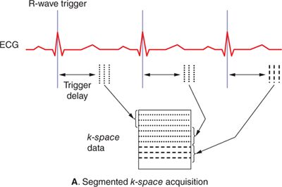
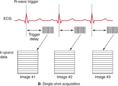
FIGURE 1-5 Segmented (A) and single-shot (B) acquisitions relative to cardiac cycle. In any segmented acquisition (A), k-space lines for each image are acquired over multiple cardiac cycles, while in a single-shot scan (B) all the data for one or more images are acquired within 1 heartbeat. While single-shot acquisitions typically require compromises in spatial resolution and signal-to-noise, they are insensitive to breathing motion and cardiac arrhythmias.
CMR TECHNIQUES
The flexibility of MRI may be more apparent in cardiovascular imaging than in MRI of any other organ system. Over the past 30 years, numerous CMR techniques have been developed for static morphological imaging of the heart and blood vessels, qualitative and quantitative imaging of motion and flow, tissue characterization based on endogenous and exogenous contrast, and even imaging of physiological parameters such as myocardial stiffness and diffusion. While a complete description of all of the various techniques is beyond the scope of this chapter, the basic pulse sequences most commonly used in clinical CMR and magnetic resonance angiography (MRA) are discussed in the following sections.
Cardiac Morphology
Any CMR exam begins with a series of rapid, large field-of-view anatomical images of the thorax often called “localizers” or “scouts.” These scout sequences are intended, as the name implies, to get a quick overview of the anatomy and provide the anatomical reference views needed to plan out subsequent scans. Exquisite detail is not required so scouts typically utilize single-shot techniques that acquire in a single heartbeat all of the k-space data needed to reconstruct an entire image. This can be accomplished easily using either a bright-blood technique such as balanced steady state free precession (SSFP) or a black-blood technique like half-Fourier acquisition single-shot turbo spin echo (sometimes called HASTE). The scans are ECG-triggered, with data acquisition timed to diastole to avoid excessive cardiac motion. Some typical scout images acquired using single-shot SSFP are shown in Figure 1-6.
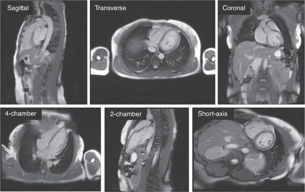
FIGURE 1-6 Array of 2D scout images in various orientations. Images are typically acquired first in straight sagittal, transverse, and coronal orientations (top row) with large fields-of-view to get a general overview of the location and orientation of the heart. This is followed by a series of targeted views to arrive at the conventional long-axis and short-axis orientations (bottom row). The images shown were generated using single-shot SSFP; each image took approximately 300 milliseconds to acquire.
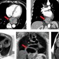
In patients with congenital heart disease, who might have potentially complicated anatomy, a 3D scout acquisition using SSFP and navigator respiratory gating may be useful for planning of subsequent views based on a full-3D volume of the thorax. This 3D data can be reformatted to define and visualize any arbitrary slice positions and orientations as shown in Figure 1-7.
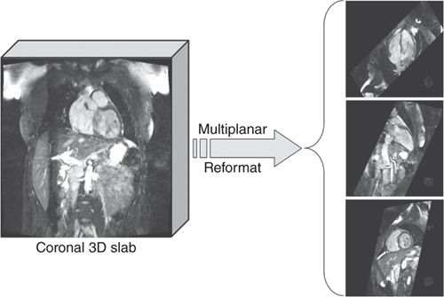
FIGURE 1-7 3D volume data showing multiplanar reformatted cut planes. In situations where the anatomy is potentially complicated (eg, patients with congenital heart disease) it can be useful to acquire a full-3D volume of the heart with near-isotropic resolution and then reformatting into the desired views. The 3D data are typically acquired using a navigator-echo respiratory gating technique to avoid respiratory motion artifact.
2D Turbo or Fast Spin-Echo
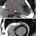
Beyond basic scout imaging, more detailed morphological imaging of the heart with specific contrast characteristics (ie, T1-weighting, T2-weighting, fat suppression) is often utilized to help characterize masses in the heart and mediastinum as well as pathological changes in myocardial tissues such as inflammation or edema. One of the first techniques developed for MRI of the heart and major blood vessels was ECG-gated spin-echo imaging with T1- or T2-weighting.6 In a spin-echo sequence, the signal from blood is naturally suppressed by flow that prevents the blood excited by the 90-degree pulse from being refocused by the 180-degree pulse.7 This “washout” effect results in black blood and provides high-contrast between the blood and myocardium, making this the preferred method for evaluation of the anatomy of the heart and major vessels. As with any spin-echo technique, image contrast can be controlled by varying the TE and TR of the sequence, for example long-TE and long-TR provide T2-weighting. The basic discovery that T2 increases with acute myocardial infarction was made in the early 1980s, not long after cardiac MRI became feasible.8,9 This finding is consistent with other tissues in the body where an acute injury leads to tissue edema, increased free water, and an elevated T2. While early techniques for T2-weighted imaging were based on a gated spin-echo acquisition; this sequence is highly sensitive to motion and image quality was unreliable. In the mid-1990s, the technique of turbo spin-echo (TSE) or fast spin echo (FSE) was introduced. In this technique, multiple 180-degree refocusing pulses are applied following each excitation pulse, enabling the acquisition of multiple lines of k-space data in each TR, thereby dramatically shortening scan time. By reducing the scan time down to a reasonable breath-hold, respiratory motion artifact can be avoided. Combining the turbo spin-echo readout with a double-inversion or “black-blood” preparation pulse (Figure 1-8) suppresses residual artifacts caused by slow flowing blood.10 A third inversion pulse with short inversion time (STIR) can be included to suppress fat and enhance sensitivity to fluid.
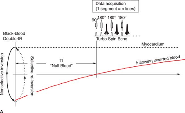
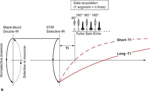
FIGURE 1-8 Black-blood turbo spin echo illustrating the double inversion recovery (A) and triple inversion recovery (B) techniques. In both of these techniques, a pair of 180-degree pulses, one nonselective and one slice-selective, is applied at the R-wave trigger. This has the effect of inverting all of the blood and tissue outside the imaged slice. Inverted blood flows into the slice and image data are acquired when the blood is near its null point. In the triple-IR sequence, a third inversion pulse is applied to suppress fat and other tissues with short-T1; this enhances the sensitivity to fluid and edema.
Related posts:
Stay updated, free articles. Join our Telegram channel

Full access? Get Clinical Tree


