Routine clinical interpretation of dynamic contrast-enhanced magnetic resonance imaging (DCE-MRI) by radiologists is based on subjective assessment of signal enhancement and the change in signal intensity as a function of time after the injection of contrast media. This chapter reviews semi-quantitative and quantitative methods that can help Radiologists to more accurately diagnose cancers by providing standardized MRI parameters that are markers for malignancy. Semiquantitative analysis of DCE-MRI data provides parameters such as rate of signal enhancement and the decay of enhancement during contrast media washout. Semiquantitative approaches are relatively simple to implement in routine clinical practice, as these approaches do not require specialized acquisitions or complicated calculations. Quantitative methods have potential to standardize diagnosis by correcting for variations in Radiologists’ expertise, scanner performance, and the systemic physiology of the patient (e.g. cardiac output). In addition, quantitative methods attempt to relate MRI measurements directly to intrinsic properties of tissue, such as blood flow and capillary permeability. In this chapter we discuss a number of widely used semi-quantitative and quantitative methods for DCE-MRI including the “three time point method,” use of empirical mathematical models, use of compartmental models, impulse response analysis, reference tissue methods, and calibration methods required for quantitative measurements.
12 Semi-Quantitative and Quantitative Analysis of Breast DCE-MRI
12.1 Semi-quantitative Analysis
Routine interpretation of dynamic contrast-enhanced magnetic resonance imaging (DCE-MRI) by radiologists is based on signal intensity and the change in signal intensity as a function of time after the injection of contrast media. Semi-quantitative techniques aid lesion categorization and provide excellent diagnostic accuracy in breast DCE-MRI. Semi-quantitative analysis has the advantage of being relatively simple to implement in routine practice, as approaches predominantly focus on postprocessing of standard clinical images and do not require specialized acquisitions.
The three time-point (3TP) method is a simple tool for classification of signal intensity time-course curves. The 3TP takes the first time-point in the DCE series, a “peak intensity” time-point (generally chosen roughly 2 minutes postcontrast administration), and a delayed time-point (approximately 6 minutes postcontrast). 1 Discrete thresholds are then used to classify two parts of the kinetic curve, the initial uptake and the delayed phase. An example of the types of classifications is illustrated in Fig. 12‑1. The classification data can then be displayed as a color overlay (on a voxel-by-voxel basis) on the standard images on computer-aided visualization stations. 2 For example, red, green, and blue color overlays can be placed on voxels displaying washout, plateau, and persistent delayed kinetics, respectively. The color intensity can also be adjusted to reflect the initial rise depending on whether it was slow, medium, or rapid. This provides radiologists a way of visually assessing the kinetics of lesion without the need to manually draw a region of interest (ROI). Kelcz et al evaluated the performance of observers aided by the 3TP in the detection of breast cancer, and found that this method had a sensitivity of 87% and specificity of 84%. 3

While the discrete categorization of lesion kinetics has been shown to be diagnostically useful, previous work by Jansen et al 4 found that the BI-RADS descriptors of curve shape can vary significantly between different scanners and acquisition parameters in malignant lesions. Thus, results obtained with methods such as the 3TP may be inconsistent across different sites, as its performance will depend on the particular thresholds chosen.
Chen et al 5 used a robust, automated, segmentation method to find the region of a lesion with the highest initial enhancement. Four kinetic features were extracted from this region in each lesion: maximum enhancement, uptake rate, washout rate, and time to peak enhancement (TTP). TTP was defined as the time when the maximum signal enhancement was measured. Uptake and washout rates were determined from TTP and the maximum enhancement. Chen et al found that accuracy of classification was greater for automated segmentation than manual placement of ROIs. Of these features, TTP had the greatest area under the receiver operating characteristic (ROC) curve (0.85 ± 0.04); the values for uptake and washout rates were 0.71 ± 0.05 and 0.79 ± 0.05. These results suggest that these kinetic features may be diagnostically useful in the categorization of lesions.
The signal enhancement ratio (SER) was introduced by Hylton and co-workers as a way of quantifying lesion kinetic curve shape on a continuous scale. 6 The definition of SER is based on the standard interpretation of curve shape. SER is defined as:
where S 0 is the precontrast or baseline lesion signal intensity, S early is the signal intensity measured at the early postcontrast phase (roughly 1–2 minutes postinjection), and S delayed is the signal intensity at the delayed phase (~6 minutes postinjection). SER can be thought of as a descriptor for curve shape because it indicates whether the transition from uptake to washout has occurred before, during, or after the time interval marked by S early and S delayed. SER has been shown to have diagnostic utility with a previous study reporting a sensitivity of 95%; specificity, however, was 47%. 7 SER has also been reported to be useful for evaluating tumor response to therapy, and has been shown to correlate with a parameter associated with tumor physiology (redistribution rate constant k ep). 8 , 9 , 10 These results show the potential value of SER added to standard clinical practice. SER, however, is affected by the particular times at which the early and delayed phases are measured; as a result, temporal resolution will have an effect on the measured SER.
Time to enhancement (TTE) is another nonparametric semi-quantitative measure that may be of clinical utility. As its name suggests, TTE measures the time at which lesions first begin to enhance significantly. However, in order to reliably measure TTE, high temporal resolution imaging is necessary. One advantage of measuring TTE from fast acquisitions is that this allows measurement of TTE relative to the time at which the contrast bolus first reaches the breast, reducing dependence on variables such as cardiac output and leading to estimates that are more descriptive of lesion physiology. In a pilot study by Pineda et al 11 with images acquired with 6- to 10-second temporal resolution, TTE was found to be significantly different between benign and malignant lesions, with average values of 15.5 and 6.9 s after arterial enhancement in the breast, respectively. Mus et al 12 evaluated the utility of TTE (measured relative to the time of aortic enhancement) in a retrospective study with images acquired with 4.32-s temporal resolution. They found that TTE had a significantly better discriminative ability than kinetic curve type. Using a TTE threshold of 12.96 s to classify lesions (lesions below this threshold were considered malignant), the authors found an AUC as high as 0.86 using TTE alone.
12.2 Empirical Mathematical Models
As an alternative to pharmacokinetic model approaches, pure mathematical models are also common for analyzing the DCE-MRI data. These pure mathematical models make no assumptions about the underlying physiology of a tumor, but simply use functions with limited parameters to characterize the important features of contrast agent uptake and washout curves as a function of time. The mathematical models are used as a tool to smooth the signal enhancement versus time curves and interpolate the data. This approach may be advantageous because tumors are extremely heterogeneous and simple compartment models may not be consistent with the true spatiotemporal distribution of contrast agent molecules in the tumor microenvironment. For example, the two-compartment model is not consistent with initial rapid uptake of contrast media followed by a slower, more prolonged uptake phase. For noisy and/or low temporal resolution DCE-MRI data, the use of fitted curves based on empirical mathematical models (EMMs) facilitates calculation of arterial input functions (AIFs) from reference tissues, 13 , 14 , 15 improves measurements of physiological parameters, and facilitates calculation of the “area under the curve” of enhancement versus time, TTP, and initial uptake slope.
Several mathematical models have been developed for analysis of DCE-MRI data. Fan et al developed a five-parameter EMM to analyze DCE-MRI data from animal models of prostate cancer and human breast cancer. 15 , 16 This EMM yields five parameters descriptive of lesion kinetics. A modified three-parameter EMM was introduced by Jansen et al to describe signal enhancement of lesions in clinical breast DCE-MRI. 17 , 18 In the three-parameter EMM, percent signal enhancement (PSE) as a function of time is given by:
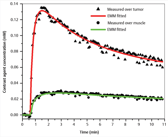
where A is the upper limit of enhancement, α is the uptake rate (per minute), and β is the washout rate (per minute). The EMM also allows calculation of secondary parameters such as the TTP, initial slope, and the initial area under the contrast curve. In a study that analyzed 100 patient scans with the EMM, it was shown that several of the primary and secondary parameters varied significantly between benign and malignant lesions. 17 Some of the EMM parameters also showed significant differences between tumor subtypes. The EMM was shown to have the potential of increasing the specificity of DCE-MRI with respect to BI-RADS descriptors of curve shape. The EMM has the added benefit of providing continuous variables for lesion classification; this means that thresholds can be adjusted to achieve desired sensitivity and specificity, as opposed to discrete classification of curve shape. Another class of functions that are commonly used to describe the signal increase in DCE-MRI are modified logistic functions (or sigmoid curves). Moate et al 19 [REF] proposed using a five-parameter modified logistic equation to describe signal enhancement in breast tumors, and demonstrated that parameters from this model have diagnostic value for analyzing breast DCE-MRI. Platel et al 20 used this model to fit the enhancement during an ultrafast DCE-MRI acquisition. Orth et al 21 used two modified sigmoids to fit the data from a dual tracer experiment in a preclinical model of breast cancer. While these functions have been shown to fit the shape of enhancement curves, the relationship between individual parameters and the shape of the curve is not entirely straightforward, and the inclusion of more parameters in the model means that more data along the signal time-course are required to obtain accurate fits. Gliozzi et al 22 used an “extended phenomenological universalities” (EU1) approach to analyze signal intensity versus time curves. Among these pure mathematical models, the EMM provides optimal fits to experimental DCE-MRI data and can be used to fit a range of contrast agent concentration versus time curves. Fig. 12‑2 shows an example of EMM fits (red and green lines) to contrast agent concentration curves obtained from a rat model for prostate cancer (AT2.1 prostate cancer) (triangles) implanted in the hind limb and normal leg muscle (dots) acquired at 4.7 T.
12.2.1 Quantitative Analysis
Data Acquisition Methods
This section discusses acquisition techniques used to obtain information required for standardized, quantitative analysis of DCE-MRI data, specifically native T1 measurements and maps of the transmit radiofrequency (RF) field (or B1). This information can also be used to correct semi-quantitative parameters. These measurements are not part of most routine, clinical, DCE-MRI acquisitions, because routine clinical analysis is generally based on qualitative interpretation of the images. However, quantitative methods are increasing in popularity, because they allow standardized measurements that can be compared across different scanners, sites, and patients.
T1 Mapping
Accurate T1 maps are essential for accurate calculation of concentration of contrast media as a function of time in each image voxel (discussed later in this chapter). Here, we summarize some of the most commonly used methods for mapping T1. This summary is not by any means an exhaustive list of T1 mapping methods.
Spoiled Gradient Echo with Variable Flip Angles
This is one of the most widely used T1-mapping methods for breast MRI. Data are acquired using a series of spoiled gradient echo images with variable flip angles (VFAs). 23 The measured signal in each voxel is then fit to the gradient echo signal model as a function of flip angle, to obtain an estimate of T1:
where θ is the flip angle, TE is the echo time, and T 2 * is the transverse relaxation time. Variations in the signal in equation (3) as a function of flip angle depend on TR, a known parameter, and T1 . The VFA method allows acquisitions of T1 maps across a large volume with reasonable scan times. The accuracy of the VFA method is influenced by the accuracy of the flip angles used in equation (3), the choice and number of flip angles, and the noise present in the images. 24 , 25 Actual flip angles can vary spatially across the field of view (FOV), and differ significantly from the angles prescribed at the scanner console, due to an inhomogeneous transmit RF field (or B1 field). This issue is discussed later in this chapter. Cheng and Wright showed that a bias of up to 10% in estimated T1 can be introduced when three flip angles are used and the signal-to-noise ratio (SNR) is 150 in the VFA data (TR = 5 ms). 26 They also showed that the VFA method can be tailored to provide accurate estimates of T1 within a narrow range when two flip angles are used. Adding more than two flip angles provides better results over a wider range of T1 values. Interestingly, simulations by Cheng and Wright showed that use of 10 different flip angles does not increase the performance relative to use of 3 angles, likely due to the influence of adding noisy data points (i.e., at lower flip angles). With judicious selection of flip angles, 25 and knowledge of the B1 field, the VFA method can provide accurate T1 maps with reasonable acquisition times, making it a suitable method for use in addition to standard clinical breast protocols.
Inversion Recovery Measurements
Inversion recovery (IR) is widely regarded as a very accurate T1 mapping method and is commonly used to measure “gold standard” T1 values. 27 In an IR sequence, a 180° pulse is first applied, inverting the spins and thus the net magnetization. The rate at which the spins recover to their initial alignment is determined by their T1. This means that measurements of magnetization as a function of time after the inversion pulse leads to an estimate of T1, derived from the IR signal model:
where M(TI) is the magnetization measured at a given inversion time “TI,” TR is the repetition time, and M 0 is the equilibrium magnetization. An additional parameter can be included in equation (4) to account for imperfect inversion pulses (i.e., not exactly 180°). The main drawback of using IR for T1 measurements is the long acquisition times it requires. For accurate estimates of T1, TR must be sufficiently long for magnetization to return to equilibrium following the inversion pulse (i.e., TR ≫ T 1). 28 A commonly used rule of thumb is that TR should at least be five times the longest T1 being measured. The long acquisition times of IR make it ill-suited for application in routine clinical scans, especially in the case of the breast, where large FOVs are necessary for full bilateral acquisitions. To overcome this limitation of IR, sequences such as Look-Locker inversion and modified Look-Locker inversion (MOLLI) have been developed. 29 , 30 These sequences allow accelerated acquisition of T1 maps in cardiac imaging, where fast acquisitions are critical. However, application of these sequences has been limited to areas of the body where small FOVs are used; thus, there is a lack of evidence about their applicability and accuracy for breast imaging.
Reference Tissue Method for T1 Measurements
Medved et al 31 showed that, under certain conditions, the T1 for a tissue of interest can be calculated from the signal of a reference tissue (i.e., a nearby tissue with a known T1). The advantage of this method is that if a tissue with a homogeneous T1 (low intra- and interpatient variability) is present in the FOV, a full T1 measurement may not be necessary, reducing total scan time. This method relies on the fact that in a gradient echo acquisition, the product of signal × T1 is approximately constant (S×T1≈constant)S\times {T}_{1}\approx constant) if the flip angle used is greater than 30° and if the repletion time (TR) of the acquisition is much shorter than the T1 values of the tissues being imaged, so that magnetization is highly saturated. This means that if differences in T2* between the reference tissue and the tissue of interest are relatively low (a realistic assumption outside the brain), and the MRI-detectable proton density between the two tissues is roughly the same, the following relationship can be used to obtain the T1 for a tissue of interest with a single gradient echo acquisition:
where S is the signal measured in a given voxel and the subscript “ref” indicates the reference tissue. In the breast, fat is an ideal reference tissue, since it has a homogeneous T1. Reported values for the T1 of breast fat include 265 ± 2 ms 32 and 230 ± 10 ms, 33 both at 1.5 T. At 3 T, Rakow-Penner et al 34 reported a value of 367 ± 8 ms, and Pineda et al 35 measured a T1 of 341 ± 31 ms. The relatively low standard deviation in these studies, and the similar values from different studies at the same field strength, suggests a low variability in the T1 value of fat, both interpatient and across the breast. The reference tissue method is the simplest (and potentially fastest) method to measure T1, but if the conditions mentioned above are not met, significant errors in the estimated T1 values may result (e.g., if a low flip angle is used).
B1 Mapping
Transmit RF field (B1 or B1 +) inhomogeneity is especially notable in breast MRI, due to the large FOVs required for bilateral breast imaging and the off-center (with respect to the center of the magnet) position of the breasts in the coil. Kuhl et al reported significant differences in the B1 field across the FOV, with differences of nearly a factor of 2 between the left and right breasts. 36 These differences can lead to variations in image intensity across the FOV (e.g., shading), spatial variations in the signal enhancement in lesions after the administration of a contrast agent, and inaccurate T1 values measured with a VFA sequence. Azlan et al mapped the B1 field in several healthy volunteers at 3 T and simulated differences in enhancement due to B1 gradients in a phantom study. 37 They found significant differences between the right and left breasts, and reductions of more than 50% relative to the nominal B1 in some cases. They also showed that a reduction in B1 leads to a reduction of the SER, possibly reducing the conspicuity of breast lesions. While B1 inhomogeneity is an issue at all field strengths, the B1 field is more inhomogeneous at larger fields.
Dual-source parallel RF excitation, combined with RF shimming methods, has been implemented by several manufacturers to reduce variations in the B1 field. 38 Rahbar et al compared B1 maps acquired in the breast using both single and dual-source RF excitation. 39 They found that while the use of dual-source parallel excitation reduced differences in the whole breast mean B1 value between the right and left breasts compared to single-source excitation, significant differences between nominal and prescribed flip angles remained at many locations.
B1 field inhomogeneity has a significant effect on the estimation of quantitative parameters in DCE-MRI. 40 Using a VFA approach, estimation of native T1 values of tissues relies on the accurate knowledge of the flip angles used. Simulations show that for variations of up to 15% between nominal and prescribed flip angles, the relative error introduced in T1 measurements from the VFA is twice the relative error in the flip angle (i.e., a 10% error in flip angle will lead to a 20% error in the measured T1). Measurements of contrast agent concentration are obtained from the native and postcontrast-injection T1 values. They are thus affected by the errors in the estimated flip angle in the ROI. In fact, when the repetition time is short and a low flip angle is used, a small error in the flip angle can lead to a large bias in concentration. In DCE-MRI of the breast, it is common to use protocols with these conditions. For this reason, accurate knowledge of the actual flip angle is essential for accurate measurements of contrast media concentration. This section outlines B1 mapping methods that can be used in breast imaging to correct for B1 field inhomogeneity.
Actual Flip Angle Imaging
The “actual flip angle imaging” (AFI) method, developed by Yarnykh, can be used to measure B1 maps in vivo. 41 In this approach, the ratio of the signal of two gradient echo acquisitions at two different repetition times (TRs) is used to derive the actual flip angle in each voxel. When implementing this sequence, one must ensure that the transverse magnetization is adequately spoiled and that steady state magnetization has been achieved; otherwise, the accuracy of the AFI technique is affected. 42 Both TRs used in this sequence should be smaller than the shortest T1 value present in the FOV. Additionally, large flip angles (40°–80°) are required for optimal implementation of this sequence; however, this leads to a reduced SNR, potential artifacts from stimulated echoes, and a distortion of slice profiles. Some vendors offer a built-in AFI option to obtain B1 maps; otherwise, its implementation may require pulse programming knowledge.
Reference Tissue Methods for B1 Mapping
Sung et al and Pineda et al proposed using fat as a reference tissue to obtain combined T1 and B1 maps, by acquiring a VFA sequence of spoiled gradient echo acquisitions. 35 , 43 As discussed above, fat is an ideal reference tissue in the breast because of its homogeneous T1. A flip angle correction factor (which is proportional to B1) can be calculated in a voxel if its true T1 value is known (e.g., from a population average), by measuring T1 from fitting VFA data to the gradient echo signal model (equation 3) using the nominal flip angles (those prescribed at the scanner console). This correction factor (κ) is given by:
where the subscript “t” and “m” denote the true and measured T1 values for the reference tissue (fat), respectively. In these methods, the fat voxels are identified, and a value of κ is calculated for each fat voxel. The values for the rest of the FOV (i.e., all the voxels corresponding to parenchyma) are then interpolated from the surrounding fat voxels. The VFA data are then fit to the signal model again, this time using the correct flip angle for each voxel in the breast, leading to an accurate T1 map. This method provides T1 maps close to the “gold standard” IR T1 maps, even in patients with dense breasts. 35 This method for obtaining T1 and B1 maps relies only on the assumption that the flip angle correction factor will be constant for all angles, a reasonable assumption for the range of angles typically used in a VFA sequence. 44
Other B1 Mapping Methods
Other methods for in vivo B1 mapping include the saturated double-angle method (SDAM), 45 dual refocusing echo acquisition mode (DREAM), 46 and mapping by Bloch–Siegert shift. 47 Nehrke et al compared RF shimming with DREAM, AFI, and SDAM. 48 The authors found that DREAM outperformed the other methods while significantly reducing acquisition time. Bloch–Siegert shift B1 mapping offers the advantage of insensitivity to factors such as TR, T1, and flip angle (DREAM has a weak dependence on T1 and T2), and has been shown to improve the accuracy of longitudinal T1 measurements in the breast. In fact, there is potential to combine DREAM and Bloch–Siegert approaches to produce a new and more accurate method. One drawback of the DREAM and Bloch–Siegert B1 mapping methods is that they require specialized sequences that are implemented through research software patches that are not currently widely available.
12.3 Calculation of Contrast Media Concentration
While the signal in a postcontrast DCE-MRI acquisition is a function of the concentration of contrast media, other factors affect the amount of signal enhancement in these images. The shortening of T1 values in the presence of contrast media is described (in the fast-exchange regime) by the following equation:
where T1(c) is the T1 in the presence of a concentration “c” of contrast media, T10 is the native T1 of the tissue in question, and r 1 is the relaxivity of the contrast media agent, a value that is well characterized in the literature for most widely used contrast media agents. Simple inspection of equation (7) shows that a tissue with a larger native T1 will have a larger change in T1 for the same concentration of contrast media (and thus higher signal enhancement in a T1-weighted image). Along with the native T1 and the relaxivity and concentration of contrast media, the TR and flip angle of the spoiled gradient echo acquisition used for DCE-MRI (as shown in equation 3) will also affect the amount of signal enhancement seen in these images. In order to obtain images that are independent of acquisition parameters and of the native T1 of the tissues being imaged, standard DCE-MR images are converted to images of contrast media concentration.
As mentioned above, the r 1 of each contrast agent can be found in the literature, 49 , 50 and the native T1 of tissues can be measured using one of the methods described above. Once r 1 and T10 are known, the final step in estimating the concentration of contrast media is measurement of the postcontrast shortened T1. Ideally, T1(c) would be measured directly by acquiring a series of T1 maps following the administration of contrast media. However, this would require very fast T1 mapping sequences, since contrast media concentration will be changing rapidly, especially in the time shortly after it is administered. In some areas of the body, where the volumes acquired are not large, this can be achieved. 51 Even if reasonably short T1 mapping techniques were to be used, many of the acquired images would not be diagnostically useful, due to inadequate SNR or image contrast (i.e., at low flip angles). The alternative is to estimate postcontrast T1 from signal changes in the routine clinical sequence and precontrast native T1 measurements. This way, the standard clinical images are used for routine interpretation, while postprocessing is used to obtain estimates of T1 at each time-point.
In a spoiled gradient echo sequence, the PSE as a function of time can be expressed as (from equation 3):
where E10 = exp(–TR/T10), E1 = exp(–TR/T1), T10 is the native T1, T1 is the postcontrast value, and we make the common simplifying assumption that T2* relaxation can be neglected. Equation (8) can be solved to obtain a nonlinear analytic solution for T1:
Equation (9) shows that it is possible to estimate postcontrast T1 from the signal enhancement measured in a standard clinical sequence, the actual flip angle, and the native T1. The value of postcontrast T1 can then be inserted into equation (7) to obtain an estimate for the concentration of contrast media at each time point.
An alternative, and simpler approach, is to use a reference signal to estimate changes in T1 (as described in the T1 mapping section above). 15 , 31 As explained above, this method relies on the presence of a “reference tissue” with a known, and homogeneous, T1 in the FOV and the following assumptions: TR < T1, a sufficiently large flip angle (greater than 30°), and differences in T2* between the reference tissue and the tissue of interest are assumed to be low. Under these assumptions, the product of signal and T1 is approximately constant (S × T1 ≈ constant). Therefore, changes in signal are directly and linearly related to changes in T1. Under these conditions, the concentration of contrast media as a function of time can be written as:
With the reference tissue method, concentration of contrast media can be calculated from signal changes in the DCE-MRI images and knowledge of the native T1 of a reference tissue, either by direct measurement or by using a population average. This approach has been implemented using the liver and muscle as reference tissues, 31 and in the breast using fat as a reference. 15 Besides the conditions listed above, this method relies on the flip angle being the same at the tissue of interest and the reference tissue. Variations in the B1 field across the relatively large FOV used in breast imaging may limit its accuracy in the breast.
12.3.1 Arterial Input Function
The AIF is the contrast media concentration (C A(t)) as a function of time in the arterial blood supply following intravenous injection. The local AIF is C A(t) in local arteries feeding a suspicious lesion or a specific portion of the body, e.g., the internal mammary artery. Calculation of physiologic parameters such as K trans from compartmental models (e.g., the two-compartment model) requires accurate measurement of the AIF.
The contrast media AIF can vary significantly for a single subject scanned at different times and between subjects. Variations in cardiac output are a major contributor to variability in the AIF. In healthy individuals, cardiac output varies from 4.0 to 8.0 L/minute, 52 and in patients who are not in good health, the range can be even larger. The local AIF near a cancer may be even more variable. Fan et al 14 showed that in tumors grown on rat hind limb, the standard deviation of the peak amplitude of the local AIF measured using a reference tissue and artery was about 40% of the mean (n = 8). Yang et al 53 showed large interpatient and intrapatient variability in the AIF in bone metastases using a multiple reference tissue method. For the area under the first pass of the AIF, the within-subject coefficient of variation (relative standard deviation) was 11% (range, 0.2–20.8%) and the between-subject coefficient of variation was 24%, with values ranging from approximately 50 to 200% of the mean. Lavini and Verhoeff 54 demonstrated that the AIF measured directly in the superior sagittal sinus has a very large interpatient range, with relative standard deviation of AIF amplitude of 57% or higher (depending on protocol) and a range of a factor of 5. These data demonstrate that there are large variations in the AIF that can produce diagnostic errors as well as large errors in quantitative parameters derived from contrast media enhancement kinetics, such as K trans and ve (contrast media fractional distribution volume) if they are not properly accounted for. In some patients (especially the many who are more than one standard deviation from the mean), these errors will result in cancers missed by MRI, while in other patients benign lesions will be misdiagnosed as having high perfusion/permeability characteristic of cancers.
Several approaches are used to measure the AIF:
Population AIF
Population AIFs have been constructed from measurements of the arterial concentration of contrast media in multiple patients and producing a population average. A convenient functional form of the AIF can be used for quantitative analysis of DCE-MRI data, e.g., as part of two-compartment analysis. The most commonly used population AIF was developed by Parker et al 55 using the sum of two gaussian functions plus an exponential modulated by sigmoid function to model the AIF with both the first and second passes:
Related posts:
Stay updated, free articles. Join our Telegram channel

Full access? Get Clinical Tree


