8.2.1 General

Net Brownian movement of water molecules (e.g., spins, protons, or, more correctly, “water protons”) can be characterized by a diffusion coefficient, D, a variable relating the concentration gradient to the rate of transfer of water molecules through a unit of area.¹² In the brain, no appreciable water concentration gradients exist (i.e., no net flux of water); however, the concentration gradients of water in the DWI experiment can be thought of in terms of the concentration of “tagged” water molecules, similar to diffusion tracer experiments where dye is used to quantify random motion of substances. For nonrestricted diffusion, the mean displacement of a water molecule in a single dimension during time t follows Einstein’s equation.^12,​13

resulting in a Gaussian probability of displacement for a given water molecule:

where r₀ is the initial position of a specific water molecule, r is the current position, D is the diffusion coefficient, and t is time. The Gaussian probability distribution of water molecule displacement forms the basis of conventional DWI quantification.

8.2.2 Diffusion Nuclear Magnetic Resonance

The time-evolving magnetization density including nonrestricted self-diffusion of a single NMR species was first described by Torrey in 1956.¹⁴ The solution is conveniently expressed in the following form:

where the b-value represents the “level of diffusion weighting,” or attenuation, of the MR signal for a given set of DWI experimental parameters (Fig. 8.1). From Equation 8.3, we see that attenuation of the MR signal from nonrestricted diffusion of a single NMR species having a specific T₁ and T₂ characteristic follows a monoexponential decay that is dependent on the experimental parameters (b-value) and diffusion coefficient, D.

8.2.3 Biexponential Diffusion MR Signal Attenuation

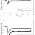
For two NMR species with similar T1 and T2 characteristics and differing diffusion coefficients (e.g., intra- and extracellular free water), MR signal attenuation is slightly more complicated. If the diffusion time, τ, the time between “tagging” and “untagging” water molecules in the DWI experiment, is slow such that there is perfect mixing between the compartments, then the MR signal attenuation is monoexponential, with a single apparent diffusion coefficient (ADC) (Fig. 8.2):

Here, S(b) represents the MR signal intensity as a function of b-value for a given echo time and repetition time, S₀ is the MR signal intensity without diffusion weighting (i.e., b = 0 s/mm²), f_in is the intracellular volume fraction, f_ex is the extracellular volume fraction, D_in is the intracellular volume fraction, and D_ex is the extracellular water fraction. For short diffusion times where minimal mixing between compartments occurs, MR attenuation is biexponential (Fig. 8.2b):

In the human brain, f_in ≈ 0.8, f_ex ≈ 0.2, and D_in < D_ex due to higher protein concentration and viscosity within the cytosol. For intermediate mixing times and compartment permeability, the solution becomes increasingly complex as described by Kärger, et al.¹⁵ As such, investigators have chosen to fit “apparent” biexponential parameters to experimental data:

where f is the volume fraction of the “fast” diffusion component, D_fast is the larger of the two diffusion coefficients typically dominating signal attenuation at low b-values, and D_slow is the lower of the two diffusion coefficients typically used to explain the residual signal intensity at high b-values. The biological basis and interpretation of biexponential diffusion, however, is still a topic of controversy.^16,​17

8.2.4 Stretched-Exponential Diffusion Imaging

These early DWI experiments in the brain resulted in new exploration of diffusion models to explain nonmonoexponential diffusion behavior. In malignant brain tumors the microenvironment is highly heterogeneous, containing a variety of cell sizes and cell shapes, having highly complex and tortuous extracellular space, and containing a wide range of water concentrations from vasogenic edema and necrosis. This can result in complex patterns of signal attenuation, such that a simple mono- or biexponential model may not be as valuable. To explain this complexity, Bennett et al^18,​19 demonstrated the utility of a continuously distributed, or “stretched,” exponential diffusion model (also known as the Kohlrausch-Williams-Watts [KWW] function, Fig. 8.3) to explain nonmonoexponential diffusion in the human brain and brain tumors. This model is described as follows:

Here, DDC is a distributed diffusion coefficient, and α is a heterogeneity index that ranges from 0 (highly heterogeneous) to 1 (low heterogeneity, i.e., monoexponential decay). Investigations by Kwee et al²⁰ further suggested the heterogeneity index may be sensitive to early microscopic tumor invasion, although histological validation has not yet been performed.

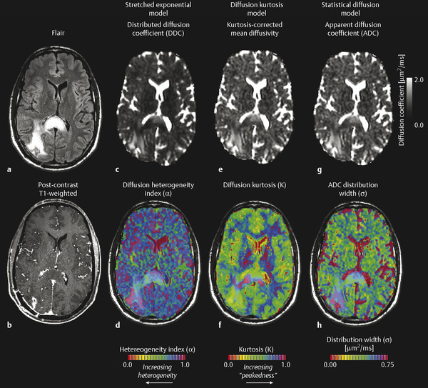
8.2.5 Diffusion Kurtosis Imaging (Isotropic)

Similar to the stretched-exponential model, Jensen et al²¹ described a “diffusion kurtosis model,” in which the first two terms of a Taylor series expansion of the logarithm of the signal with respect to b is performed, resulting in the following description of diffusion-induced MR signal attenuation:

where D is the kurtosis-corrected estimate of the diffusion coefficient and K is the “kurtosis excess,” or “peakedness of the diffusion distribution.” A recent study by Van Cauter et al²² has suggested increasing diffusion kurtosis with increasing malignancy in gliomas. Additionally, a statistical model for diffusion-attenuated MR signal was proposed by Yablonskiy et al,²³ in which the total MR signal is described in terms of a probability distribution of ADC values arising from multiple water species. The model is described by the following:

where σ is the width of the ADC distribution estimate and has been shown to be on the order of 36% of ADC magnitude.

8.2.6 Quantitative Q-Space Imaging

Although probing the subvoxel environment using multiple b-value DWI can elicit important information about the complex tumor microstructure, many of these models assume water undergoes free, nonrestricted movement within the tissue environment. Using a technique in many ways analogous to X-ray crystallography, q-space imaging (QSI) or diffusion spectral imaging (DSI) is a molecular imaging technique that uses the properties of restricted diffusion to quantify a water displacement profile. Simply stated, water molecules will diffuse a mean distance for a given diffusion time and diffusion coefficient according to Einstein’s equation. If this distance is longer than the boundaries of a compartment restricting diffusion of the water molecule, these molecules will reflect off the boundaries and result in an increase in MR signal amplitude as water molecules approach their original position (Fig. 8.4). If the MR signal amplitude is recorded for increasingly longer diffusion times, harmonics appear in intervals related to the mean compartment size. Taking the Fourier transform of the resulting q-space spectrum results in a water displacement probability density function for each image voxel, typically on the order of micrometers. Fig. 8.5 illustrates this phenomenon.

8.3.1 Diffusion Measurement with NMR

At the most fundamental level, diffusion weighting of MR images requires phase labeling of water molecules at an initial time point using magnetic field gradients, followed by phase refocusing after a certain diffusion time later using the same gradients. The simplest method of employing diffusion sensitivity is through the use of bipolar diffusion sensitizing gradients applied to a gradient-recalled echo (GRE) experiment. A monopolar continuous gradient can be applied to a spin-echo (SE) experiment, resulting in the same expression for b-value. In 1965, Stejskal and Tanner introduced the pulsed gradient spin-echo (PGSE) diffusion encoding scheme,^1,​2 which is still one of the most popular sequences used in clinical DWI. The PGSE experiment differed from previous techniques in that a diffusion mixing time, Δ, was introduced into the experiment. More exotic diffusion encoding schemes have also been developed for use in clinical DWI. For example, Reese et al²⁴ recently developed the twice-refocused spin-echo method for diffusion preparation, which reduces eddy-current-related artifacts by introducing additional refocusing pulse and reversed polarity gradients. This sequence is now widely available on clinical scanners, but it has the disadvantage of relatively long echo times compared to other PGSE sequences. Another example of a rather common, more advanced diffusion encoding scheme is a stimulated echo acquisition mode (STEAM) PGSE, which is useful for reducing the long echo time requirements for long diffusion mixing times (Δ). In the STEAM-PGSE encoding scheme, transverse magnetization from the initial excitation pulse is tipped 90 degrees into the longitudinal orientation, where the magnetization vector decays according to the T1 relaxation instead of the shorter T2. At some later time, τ, the magnetization is tipped back into the transverse plane, the spins are refocused using the diffusion sensitizing gradients, then the spin-echo is acquired. Yet another example of an exotic diffusion encoding scheme that is clinically useful is the oscillating-gradient spin-echo (OGSE) sequence, which can be used to probe very small diffusion times while maintaining relatively large b-values.

8.3.2 Acquisition Techniques

Traditional PGSE diffusion MRI requires a single diffusion preparation per line of k-space. Although this is the simplest method of performing diffusion MRI and the method that results in the highest overall signal-to-noise ratio, it is not clinically feasible due to long acquisition times and high sensitivity to bulk motion between acquisitions. Scan time for traditional PGSE DWI can be approximated by the following:

Related posts:

7 Perfusion Imaging: Perfusion CT 6 Perfusion Imaging: Arterial Spin Labeling 1 Conventional Morphological Imaging: MRI Remains the Workhorse 15 Image-Guided Neurosurgery: Intraoperative MRI 18 On the Horizon: Going Beyond Conventional MR Contrast Agents 13 It’s Not Just the Tumor: Treatment Effects

Stay updated, free articles. Join our Telegram channel

Join