Advanced Methods for IVIM Parameter Estimation
This chapter reviews the difficult problem of parameter estimation in intravoxel incoherent motion (IVIM) modeling and attempts to summarize the various advanced approaches that have been proposed to improve the precision and accuracy of the pseudodiffusion parameter estimates.
23.1 Introduction
Parameter estimation by fitting a biexponential model to noisy data is a notoriously difficult problem [1–5]. Using synthetic data and nonlinear least squares (NLLS) curve fitting, Bromage [1] showed that estimation error (relative to data error) increases substantially as the amplitudes of the exponential components become increasingly dissimilar. Unfortunately, this is precisely the situation in IVIM imaging studies, where the pseudodiffusion volume fraction, f, is often in the range 5%–10% [6] and is generally lower than 30% [7]. As such, information about the pseudodiffusion component is contained in only a small fraction of the signal, and the measurement is said to have a poor dynamic range [8]. Of course, this situation is exacerbated by the low signal-to-noise ratio (SNR) typically encountered in diffusion-weighted imaging (DWI).
In the majority of cases, IVIM parameter estimation is performed using either NLLS fitting or an asymptotic approach, as described below. Typically NLLS fitting is implemented using either the Levenberg–Marquardt algorithm [9, 10], a trust-region algorithm [11, 12], or occasionally the Nelder–Mead simplex method [13, 14]; all of these are readily available in many data analysis programs. However, if performed on a pixel-wise basis, corresponding estimates for f, and especially the pseudodiffusion coefficient, D*, generally possess a high degree of variability, such that averaging over entire regions of interest (ROIs) is often required in the pursuit of meaningful results [7,15,16]. As such, it is generally accepted that NLLS fitting is inadequate in the pursuit of clinical IVIM imaging.
In this chapter we review the various alternative approaches that have been proposed to date for improving the robustness of IVIM parameter estimation. We begin with a brief overview of asymptotic approaches and the important task of b-value (diffusion weighting) optimization before exploring more advanced methods, focusing in particular on Bayesian inference with a variety of different priors; we also cover non-negative least squares (NNLS), total variation regularization, various noise-based approaches, and machine learning. Note that alternative models [17] and flow-compensated IVIM [18, 19] are discussed in detail elsewhere in this book.
23.2 Asymptotic Approaches
23.2.1 Simplified IVIM
While discussion of simplified IVIM may appear somewhat mis- placed in a chapter on advanced methodology, it has been includedhere for completeness and for historical reasons. Simplified IVIM is based on the assumption that the pseudodiffusion component has essentially decayed to zero for b values above a suitably high thresh- old, and this assumption also forms the basis of the segmented fit- ting approach, which is described below. In the first exposition of the IVIM model, Le Bihan et al. [20] showed that as few as three b values are required to provide estimates of the diffusion coefficient, D, and f (i.e., D* is not estimated). Taking the natural logarithm of the data, the slope of the straight line passing through the data at the higher two b values provides an estimate of D, and after rearrang- ing the expression provided by Le Bihan et al. [20], it can be shown that the difference between the vertical intercept of this straight line (S int) and the datum at b = 0 s/mm2 (S 0) can be used to estimate f = (S 0– S int)/S 0.
Acquiring data at only three b values is attractive with regard to the scan time and permits pseudodiffusion informationto be obtained at little or no cost to existing clinical protocols used for estimating the apparent diffusion coefficient (ADC). Such information has been shown to hold diagnostic value in a number of recent studies [21–23]. Several other metrics have also been proposed that essentially provide alternative weightings of the simplified IVIM parameters [24–28]. Of course, the choice of b values has a substantial impact on parameter precision and accuracy (see Fig 23.1), and the optimal choice also depends on both tissue type and SNR [28–30].
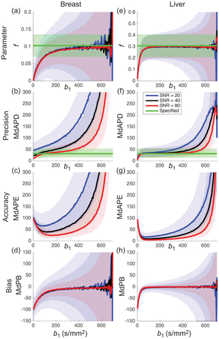
Figure 23.1 Impact of the choice of middle b value and SNR on the estimation of parameter f (shading depicts interquartile range) when applying simplified IVIM to synthetic data appropriate to the breast (a-d) and liver (e-h). Reprinted Ref. [28] with permission from Springer Nature, copyright 2017.
Possibly implicit in the use of simplified IVIM is the belief that the expected uncertainty in D* does not warrant the additional scan time necessary for its estimation [23]. An alternative approach, therefore, is simply to fix D* and solve for f and D using NLLS, which has been shown to provide more robust estimates than simplified IVIM [31]. However, in that study the observed improvement was arguably primarily due to the additional b values sampled rather than differences in methodology.
23.2.2 Segmented Fitting
The framework behind simplified IVIM can be extended easily to incorporate multiple b values above the assumed threshold, thereby improving the robustness of the estimates for f and D [32, 33]. This approach has been shown to provide more stable estimates of f than NLLS, even when using the asymptotic estimates as the starting values for NLLS [34]. Note that the fitting can be performed either by applying weighted least squares to the log-transformed data or by applying NLLS with a monoexponential model.
Segmented fitting extends this idea further by also solving for D* by applying NLLS using the full biexponential model after first fixing f and D to the asymptotic estimates [35]. Alternatively, one can solve for both f and D* using NLLS after fixing only D [36]. The argument is that the stability of NLLS is improved by reducing the number of parameters to be estimated. Note that a check should be included to ensure that the signal at higher b values has not yet reached the noise floor, which would otherwise heavily bias the estimates of f (increase) and D (decrease) [37].
Segmented fitting has been compared extensively against full NLLS, and while full NLLS by definition should provide a better fit to the data (i.e., lower residual sum of squares), the estimates of the pseudodiffusion coefficients provided by segmented fitting generally contain fewer outliers and have lower coefficients of variation [6,38–43]. However, when comparing the approaches using median statistics, which are themselves less susceptible to the existence of outliers and therefore arguably more representative of the bulk of the data, studies have shown the full NLLS approach (trust-region) in certain simulations to be slightly superior [44, 45].
The estimates for f and D obtained using segmented fitting are always biased to a certain extent because of the finite pseudodiffusion component that is still present in the signal at the threshold b value, and the influence of the choice of threshold is highly tissue dependent. Rather than fixing the threshold for a given study, Wurnig et al. [46] proposed an automated approach whereby segmented fitting is applied multiple times using every possible threshold from the available set of b values, and the one providing the best fit to the data is used for determining the parameter estimates (see Fig 23.2). Indeed, this optimal threshold has also been proposed as a possible biomarker in its own right [47].
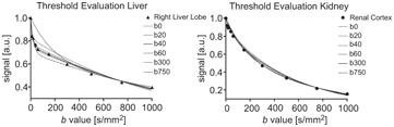
Figure 23.2 Impact of the choice of threshold b value on the resulting biexponential curve when applying segmented fitting to liver and kidney data (best fit using thresholds at b = 40 s/mm2 and b = 300 s/mm2, respectively). Reprinted from Ref. [46] with permission from John Wiley and Sons, copyright 2014.
A number of variants to segmented fitting have been proposed. For example, the second step of solving for D* using NLLS can be replaced by further linearized least squares fitting using either a Taylor series approximation at low b values [48] or transformed data [45]. A variable projection approach has also been proposed that bears some similarities to segmented fitting in that it reduces the parameter space by first solving a linear equation for f [49]. The algorithm requires initial guesses for D and D*, followed by iteration involving NLLS at each step.
23.3 b-Value Optimization
Given the sensitivity of the IVIM parameters to both the SNR of the underlying data and the chosen method of estimation, it is reasonable to expect that the number and distribution of b values are also important factors. Hence b-value optimization has become an important means to improve the robustness of IVIM parameter estimation.
Lemke et al. [7] considered three perfusion regimes correspond- ing to brain (low), kidney (medium), and liver (high) tissue and used Monte Carlo simulations to generate synthetic noisy data sets. These authors started with three fixed b values and successively added b values that minimized the relative overall error of the parameter es- timates (obtained using the Levenberg–Marquardt algorithm). Thus, an ordered set was presented, and a minimum of ten b values was recommended. Histogram analysis showed that optimal b values were concentrated within three broad clusters. A similar approach has been applied to the optimization of b values for other diffusion models [50].
Zhang et al. [51] derived an error propagation factor equal to the ratio of the relative parameter error to the relative input noise (assuming NLLS fitting). A weighted sum of error propagation factors for each parameter was integrated over parameter ranges appropriate to the kidney and then optimized with respect to 4, 6, 8, and 10 b values. The optimal distributions involved repeated sampling at key b values and afforded improved precision and accuracy over the use of a uniform distribution of b values. Cho et al. [40] tested such an optimal distribution on synthetic and in vivo data of the breast and found that it generally resulted in lower relative error compared to a more conventional distribution, both for NLLS and segmented fitting, with the latter approach being preferred.
Cohen et al. [52] considered a conventional distribution and demonstrated the importance of including at least two additional low b values between 0 and 50 s/mm2 for the estimation of D* using segmented fitting of liver data, with respect to bias and the number of outliers.
Dyvorne et al. [53] considered a model-free approach by using in vivo liver data sets comprising 16 b values along with exhaustive sampling to find the optimal subsets of 4–15 b values in terms of a global parameter error (relative to reference estimates obtained using all 16 b values). These authors found that as few as four optimal b values yielded parameter estimates with deviations lower than the repeatability deviation of the full 16 b-value set (using NLLS).
In contrast, ter Voert et al. [54] found that a minimum of 16 b values was necessary for reliable results in the liver using NLLS. These authors considered three reference protocols comprising 25 b values with which to compare the results of a series of optimized subsets, obtained by considering the error propagation factor introduced by Zhang et al. [51], along with 35 other distributions found in the literature (see Fig 23.3). A substantial reduction in the average relative error was demonstrated when the number of b values was increased from 4 to 16, and especially when using an optimized 16 b-value protocol. Errors for the pseudodiffusion parameters were generally higher for inhomogeneous tumors than for normal liver tissue.
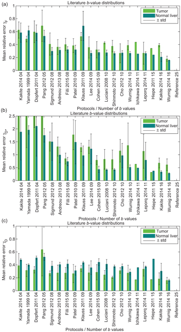
Figure 23.3 Mean relative error for f (a), D* (b) and D (c), for various b-value distributions taken from the literature, relative to a reference distribution of 25 b values, when applied to IVIM imaging of the liver. Reprint from Ref. [54] with permission from Wolters Kluwer Health, Inc., copyright 2016.
23.4 Bayesian Inference
After nonlinear least squares and segmented fitting, Bayesian inference is the third-most-common approach to IVIM parameter estimation. Bayesian inference offers several advantages over the former two approaches:
- No initial guesses are required for any of the parameters (i.e., there is no risk of getting stuck in a local minimum).
- A measure of uncertainty is obtained for each parameter in the form of a probability distribution.
- It is possible to incorporate prior information or assumptions to influence the parameter estimation.
A possible disadvantage is the greater computational complexity in terms of both implementation and processing. Additionally, special care must be taken when specifying prior information so as not to bias the results unduly.
Bayesian inference has found application across a broad range of disciplines, and there exist many excellent textbooks devoted to the subject [55, 56]. The aim is to calculate (or sample) a joint posterior distribution, P(q|data), which gives the probability that the parameters in the set q are “true” given the observed data. According to Bayes theorem, this posterior distribution can be expressed as follows:
(23.1)
where P(data|q) is the likelihood of observing the data given q, P(q) is the supplied prior distribution for q, and P(data) is referred to as the evidence and acts as a normalization term (this is often ignored, and the equality in Eq. 23.1 is replaced with a proportionality).
The probability distributions for the individual parameters are obtained via a process called marginalization, whereby the joint posterior distribution in Eq. 23.1 is integrated with respect to all of the other parameters over appropriate domains. Typically, this integration must be performed numerically, and often, the distribution is sampled approximately using, for example, a Markov chain Monte Carlo approach [57]. Such marginalization may also be required for dealing with so-called nuisance parameters, such as the noise variance in the data [58].
Therefore, several choices need to be made in applying Bayesian inference to IVIM data, such as:
- The noise model used in calculating the data likelihood (e.g., Gaussian or Rician)
- The form of the prior distribution (see below)
- The central tendency measure used to provide the parameter estimates (e.g., mean, median, or mode)
- The computational process for calculating or sampling the probability distributions, for which the options may depend on the other choices above
In the following text, we summarize the various choices that have been made to date in applying Bayesian inference to IVIM data, and we refer the reader to the corresponding references for precise details on implementation.
23.4.1 Non- and Minimally Informative Priors
Perhaps the simplest choice for prior distribution is to use one that does not encode any prior information (other than constraint boundaries), such as a uniform distribution. For such a prior, the joint posterior distribution in Eq. 23.1 becomes directly proportional to the likelihood function. Under the assumption of Gaussian noise, the maximum of this likelihood function occurs at the least squares parameter estimates. However, the Bayesian approach maintains the advantage that a probability distribution is calculated, rather than iterating toward a locally optimal solution from an initial guess, and hence it may be regarded as a type of robust least squares approach. An equally reasonable assumption may be to ascribe equal weighting to each order of magnitude for a given parameter, and one must also consider the manner in which to approach the constraint boundaries. Therefore, other choices of prior exist that are considered non- or minimally informative, such as the reciprocal distribution and the log-normal distribution [59]. These priors also encode little or no information except in cases where there is a high degree of data fitting uncertainty, which are associated with a broad likelihood function. Of course, such cases are not uncommon in IVIM data fitting, as outlined in Section 23.1, and hence these priors may still have considerable influence over the parameter estimates (see Fig 23.4) [59].
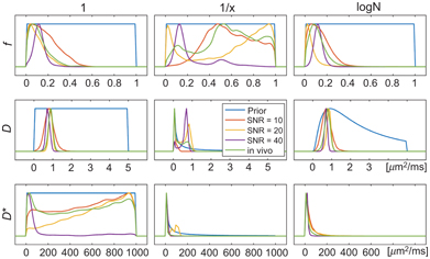
Figure 23.4 Demonstration of the impact of prior distribution (uniform, reciprocal, log-normal) and SNR on the posterior distribution (and corresponding parameter estimates) for simulated and in vivo data examples. Reprinted from Ref. [59], with permission from John Wiley and Sons, copyright 2017.
The application of Bayesian inference to IVIM data was first demonstrated by Neil and Bretthorst [8] and Neil et al. [60], who considered a Gaussian likelihood function and a prior distribution that was uniform in f and reciprocal in D and D*. The joint posterior distribution was integrated numerically, and the maxima of the marginalized distributions were used to provide the parameter estimates. These authors used simulations and rat brain data to show that Bayesian inference provided more accurate and more precise estimates than NLLS in certain cases (e.g., for D and f at a low SNR and for D* at a high SNR).
Variants of the approach by Neil et al. [8] using non- or minimally informative priors have been used inarange of IVIM studies assessing, for example, the impact of gradient polarity [61], techniques for dealing with respiratory motion [61–63], field strength dependence in the brain [64] and upper abdomen [65, 66], intrasite [67, 68] and intersite [66] reproducibility, correlation with dynamic contrast– enhanced magnetic resonance imaging (DCE MRI) in the kidney [69] and liver [70], and drug efficacy in terms of renal function [71].
However, despite the alleged improvement in robustness of the Bayesian approach over NLLS and segmented fitting, the parameters f and D* still show poor repeatability and high variability in some studies [61,63,65–68]. Indeed Li et al. [72] presented a literature review of IVIM studies in the liver and could not conclude which approach was superior, with the parameters f and D* estimated by the Bayesian approach displaying a higher median coefficient of variation across studies.
Nevertheless, the only two studies to date reporting direct comparisons between these approaches have both found that Bayesian inference with a non- or minimally informative prior does indeed provide IVIM parameter estimates with higher accuracy and precision than the other approaches [8, 44]. Barbieri et al. [44] compared six approaches: Levenberg–Marquardt, trust-region, fixed D*, two versions of segmented fitting, and Bayesian inference, using both simulations and data from the upper abdomen (see Fig 23.5). For the Bayesian inference they considered a Gaussian likelihood function, a uniform prior distribution for all parameters, slice sampling to perform the marginalization [73], and maxima to represent the parameter estimates; and they found that this approach also resulted in low inter-reader variability and the lowest intersubject variability.
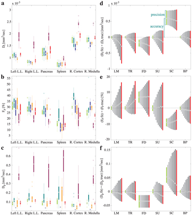
Figure 23.5 Results from experiment (a–c) and simulation (d–f) for D (a,d), f (b,e) and D* (c,f) using: the Levenberg–Marquardt algorithm (leftmost), a trust- region algorithm, fixed D*, two segmented approaches, and Bayesian inference with a uniform prior (rightmost). Reprinted from Ref. [44] with permission from John Wiley and Sons, copyright 2015.
Gustafsson et al. [59] presented recently a comparison of different approaches to Bayesian inference using non- or minimally informative priors for IVIM parameter estimation, using simulations and data from a mouse tumor model. These authors considered two different likelihood functions (Gaussian and Rician), three different priors (uniform, reciprocal, and log-normal), and two different measures of central tendency (mean and mode) and performed the marginalization using a Markov chain Monte Carlo approach [74]. The benefit of using a Gaussian likelihood function is that analytical marginalization is available, and indeed the results were found to be relatively invariant under this choice (in contrast to Bouhrara et al. [75]). However, the choice of prior and central tendency measure was found to be important (see Fig 23.6), with the log-normal prior displaying the best overall performance (using either measure).
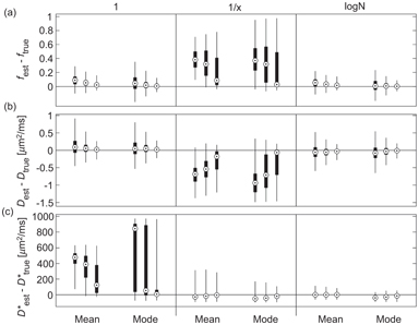
Figure 23.6 Estimation error for f (a), D (b), and D* (c), using Bayesian inference with different priors (uniform, reciprocal, log-normal), central tendency measures (mean, mode) and synthetic data SNR (10, 20, 40). Reprinted from Ref. [59], with permission from John Wiley and Sons, copyright 2017.
23.4.2 Gaussian “Shrinkage” Prior
Orton et al. [74] considered a Gaussian prior that essentially carries the assumption that the (transformed) IVIM parameters are Gaussian distributed over a ROI, which they show to be reasonable in a practical example. Specifically, they considered a hierarchical prior structure involving a multivariate Gaussian distribution for a set of transformed parameters that had been mapped onto the entire real line. Parameter estimates and measures of uncertainty were generated using a Markov chain Monte Carlo implementation, whereby at each step the Gaussian prior was redefined using the ROI mean and covariance of the parameters from the previous step. In this way, the precise shape of the prior was driven by the data themselves, and the only assumption made was that its form was Gaussian.
Orton et al. [74] also considered a Gaussian likelihood function and a conjugate Gaussian-inverse-gamma g-prior for the nuisance parameters, such that these could be marginalized analytically. Orton et al. [74] provide a detailed explanation of this Bayesian approach, along with an appendix containing all the necessary steps for numerical implementation. These authors demonstrated the approach using liver data and compared results to those obtained using NLLS (Levenberg–Marquardt). The effect of the prior was to “shrink” parameter estimates toward the mean of the Gaussian distribution for those pixels associated with a high degree of data fitting uncertainty, and this resulted in much smoother parameter maps.
While [45] presented a simulation study (breast and liver tissue) comparing the performance of this Bayesian approach using a Gaussian shrinkage prior against the use of NLLS (trust- region) and segmented fitting. The Bayesian approach was found to produce parameter estimates with consistently higher accuracy and precision than these other methods, and cleaner parameter maps. However, a possible weakness was exposed, whereby certain tissue features corresponding to regions of high data fitting uncertainty were found to disappear completely (see Fig 23.7). This finding suggests that the Gaussian shrinkage prior is best suited to ROIs that do not possess a substantial amount of underlying heterogeneity, or else it must be applied with caution and accompanied by rigorous uncertainty analysis.
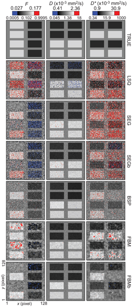
Figure 23.7 Parameter maps of f, D, and D*, for synthetic breast data, obtained using: trust-region NLLS (LSQ), segmented fitting (SEG), and Bayesian inference with a Gaussian prior (BSP) and with a spatial homogeneity prior (FBM). Reprinted from Ref. [45] with permission from Springer Nature, copyright 2017.
In line with the above recommendation for the choice of ROI, Spinner et al. [76] applied this Bayesian approach to generate IVIM parameter maps of the myocardium, which displayed lower intra- and intersubject variability when compared with the maps generated by a segmented approach, with fewer outliers for f and D*. Using simulations, these authors also showed that the Bayesian approach was associated with lower SNR requirements for the same level of bias and variation.
23.4.3 Spatial Homogeneity Prior
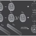
Freiman et al. [77, 78] introduced the concept of a spatially constrained incoherent motion (SCIM) model by using a spatial homogeneity prior within the Bayesian framework. The SCIM model is based on the assumption that parameter estimates in neighboring voxels should have a high probability of being similar in value. Freiman et al. [77, 78] reformulated the problem as the minimization of an energy functional involving a log likelihood term, which governs how well the parameters fit the data (noncentral c distribution), plus a spatial homogeneity term that penalizes estimates that are dissimilar to those in neighboring voxels. As such, this approach uses local information to influence the parameter estimation, in contrast to the Gaussian shrinkage prior above, which uses global information, or the priors from Section 23.4.1, which treat each pixel entirely independently. Some related approaches are given in Section 23.6, on spatial smoothing.
Freiman et al. [77, 78] also introduced the fusion bootstrap moves algorithm for solving the optimization problem. Each iteration of the algorithm comprises two steps: firstly, a new proposal (i.e., a set of parameter maps) is generated after bootstrap resampling of the data (followed by pixel-wise NLLS fitting); secondly, this new proposal is fused with the previous iteration in an optimal way using a binary graph cut that minimizes the energy functional. That is, the parameter estimates for some of the pixels in the current solution are replaced with new parameter estimates from the proposal. Additional details and references necessary for implementing this approach were provided by While [45].
Using simulations, Freiman et al. [77, 78] demonstrated reductions in root mean square error of 80% for D* and 50% for f and D, when compared with results from the Levenberg–Marquardt algorithm. These authors also applied the method to in vivo abdominal data and observed lower coefficients of variation and a higher contrast-to-noise ratio. Improved precision and accuracy was also observed in the simulation study reported by While [45], when compared to NLLS, segmented fitting, and, to a lesser extent, Bayesian inference with a Gaussian shrinkage prior (at the expense of a moderately higher bias). However, the approach was also shown to be susceptible to oversmoothing in regions of high data fitting uncertainty, in a manner similar to the Gaussian shrinkage prior (see Fig 23.7). Note that the overall degree of smoothing and the relative degree of smoothing applied to each parameter are user-defined parameters.
An adaptation of the SCIM model was incorporated recently into an approach by Kurugol et al. [79] for providing simultaneous image registration and IVIM parameter estimation. That is, this extended approach accounted for motion by also solving for the optimal transformations for each individual image. These authors actually considered a probability distribution model of diffusion instead of IVIM directly but obtained IVIM parameter estimates from this model using summary statistics. The method was applied to abdominal data and resulted in significantly improved parameter estimates when compared with the results corresponding to independent image registration.
23.5 Non-negative Least Squares
While classified here as a curve-fitting method, NNLS [80], as applied to DWI data, is essentially a generalization of IVIM in that it replaces the biexponential model with a large sum of exponential decay terms. Several hundred terms may be considered, whereby each term has a different fixed diffusion constant such that in total an appropriate range of possible values is represented (typically incremented on a logscale). The optimization problem proceeds by fitting this exponential sum to the data using regularized least squares and solving for the weights. Regularization is necessary to obtain a well-conditioned system and, for example, to enforce smoothing of the resulting diffusion spectrum.
The locations of the peaks in the spectrum provide the diffusion constants, and the relative areas under the peaks provide the corresponding signal fractions—for example, f and (1 – f) in the case of truly biexponential decay. NNLS has been used extensively in the study of nuclear magnetic resonance (NMR) relaxation data [81]. The advantage of NNLS with respect to IVIM is that it provides not only parameter estimates, but it also tests for the presence of additional decay terms that may be associated with other compartments within each voxel. Such additional terms would contaminate the parameter estimates from conventional biexponential fitting. Furthermore, NNLS does not require any starting guesses.
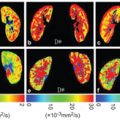
NNLS has been used to study IVIM in bone marrow [82], the prostate [83], and the brain [84] and to identify and correct for possible partial volume effects associated with large blood vessels in the liver [85]. Wurnig et al. [86] used NNLS on data obtained at as many as 68 b values to demonstrate that liver and kidney tissues are better characterized by the inclusion of a third intermediate diffusion component (see Fig 23.8). Estimation uncertainty associated with NNLS has been compared to the Cramer–Rao lower bounds for the IVIM model using Monte Carlo simulations [87].
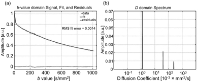
Figure 23.8 Representative data and fitted curve for liver (a), and the corresponding diffusion spectrum with three distinct peaks (b), obtained using NNLS. Reprinted from Ref. [86] with permission from John Wiley and Sons, copyright 2017.
Related posts:
 IVIM MRI: A Window to the Pathophysiology Underlying Cerebral Small Vessel Disease
 Clinical Applications of IVIM MRI to the Nervous System
 Head and Neck IVIM MRI
 Assessment of Liver Tumors with IVIM Diffusion-Weighted Imaging
 Flow-Compensated IVIM in the Ballistic Regime: Data Acquisition, Modeling, and Brain Applications
 IVIM MRI in the Kidney
Stay updated, free articles. Join our Telegram channel

Full access? Get Clinical Tree


