CHAPTER 84 Advanced Three-Dimensional Postprocessing in Computed Tomographic and Magnetic Resonance Angiography
INTRODUCTION
Automated Vessel Extraction
Segmentation and analysis of vessels in 3D image data has been an area of research for many years. In general, the definition of the vessel centerline is a first major step in the process of segmentation and analysis of vessels. Existing methods for the determination of vessel centerlines can roughly be grouped into two categories: a minimal cost path calculation;1 and methods based on first obtaining the whole set of image pixels containing the vessel (segmentation) and next gradually reducing these sets of pixels to a single centerline (skeletonization).2 The first type is typically computationally faster and avoids the error-sensitive segmentation step. However, the minimal cost path may deviate from the true lumen center at strong curvatures of the vessels. Furthermore, the intermediate result of the second type does provide some advantages such as the visual evaluation of the presegmentation of the vessel (tree).
Coronary Vessel Presegmentation
The first step in the segmentation and analysis process is a presegmentation step based on the so-called fast-marching level set method (called WaveProp for short).3 The WaveProp algorithm simulates the propagation of a wave through a medium starting from a user-selected source point, in this case the ostium of a vessel. The wave propagates through the volume set with a propagation speed given by the so-called speed function; this speed function can be designed based on image intensities in such a way that the wave propagates fast in the structures of interest (high intensities in a blood vessel) and slow in the remaining structures (low image intensities). By this image-based approach, the propagation automatically provides an initial segmentation of the vessel lumen.
Centerline Detection
The fastest path, which is the path connecting the start and end point, can be obtained using a so-called steepest-descent approach by backtracking the path of an accepted voxel in the wave propagation to the source (starting point) following the minimal travel time (highest speed). However, the fastest path tends to deviate from the center of the lumen by taking the inside curve at bending vessels. To correct the fastest path such that it follows the center of the lumen, a modified distance transformation is used.4 This distance map defines for each voxel the minimal distance to a nonaccepted voxel, and as a result, the highest values represent the center of the segmented vessels. An example is given in Figure 84-1.
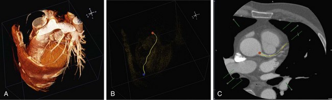
 FIGURE 84-1
Curved Multiplanar Reformatting
Because of its tortuous course and the presence of other structures such as the heart chamber, the visual evaluation of the segmented vessels may still be cumbersome. When the vessel’s centerline is known, a curved multiplanar reformatted (CMPR) image along the vessel’s course can be constructed (Fig. 84-2). The goal of CMPR visualization is to make a vessel visible in one single image over its entire length. Traditionally, two separate approaches have been used in the construction: stretched CMPR or straightened CMPR. The stretched CMPR displays a tubular structure in one 2-D plane without overlap, whereas the straightened CMPR produces a linear representation of the vessel that simulates the vessel as if it has been pulled straight. To optimize the image for contour detection, we follow the latter approach. The reformatted image contains a stack of 2D images that are perpendicular to the centerline. The third dimension, Z, in this image represents the distance to the source point along the centerline, such that the centerline is transformed into a straight line running through the X-Y center of the stack of images.
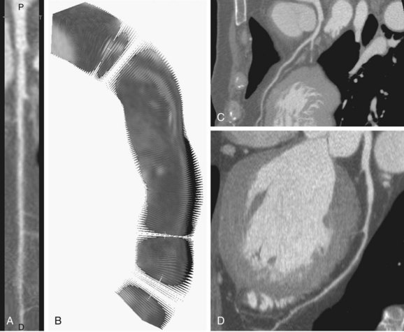
 FIGURE 84-2
Contour Detection
For the quantitative results to be insensitive to image noise, the contour detection needs to be relatively insensitive and robust to image distortions. Straight-forward contour detection methods based on thresholds of image intensities solely, second-order derivatives or the full-width half maximum method5 are sensitive to image noise, and as a result limit the algorithm to adapt to variations in the dosage or distribution of contrast agent.5 Commonly, contour detection for the determination of vessel dimensions is carried out solely on the 2D cross-sectional planes perpendicular to the vessel’s centerline. To minimize the sensitivity to image noise, we use information of the complete 3D shape of the vessel. The reformatted CMPR image enables the use of multiple 2D contour detections. For that reason, we suggest the following approach, which has been successful in IVUS applications.6
Through the stack of images, a number of longitudinal cut planes (typically 4 to 6) can be defined, which are perpendicular to the transversal planes and pass through the center of the CMPR image, and thus through the centerline of the vessel (Fig. 84-3). These cut planes are subsequently used for the contour detection along the course of the vessel.7 Experiments have demonstrated that the construction of four cut planes is sufficient for the longitudinal contour detection.
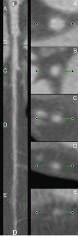
 FIGURE 84-3
The longitudinal vessel borders are detected using the model-guided minimum cost approach (MCA)8. The cost function is based on a combination of spatial first-, and second-derivative gradient filters in combination with knowledge of the expected CT values, and curvature of the coronary vessels. Because the 3D shape of the vessel resembles a smoothly curved tube, the two vessel boundaries in a longitudinal cut plane are detected simultaneously.9 This means that a well-defined vessel border at one side can support the detection of the vessel border at the other side. This mutual guidance by the simultaneous detection of the vessel boundaries is especially helpful at locations with strong partial volume effects or close to bifurcations. In these cases, the shape of the opposite contour follows the shape of the well-defined edge.
Next, the four longitudinal cut planes displaying its associated contours are presented for visual inspection (Fig. 84-4A). In some cases, such as at the presence of strong calcifications or odd branchings, manual correction of the contours may be necessary, and can easily be carried out. The longitudinal detected vessel contours produce a series of intersection points with the transversal slices. These points have two functions: (1) they are used to specify the region of interest for the MCA contour detection in the transversal images; and (2) they function as attraction points with an adjustable strength to attract the contour detection to areas close to these points. The advantage of using attraction points instead of forcing contours to run through the intersection points is that small deviations in the longitudinal contours do not force the transversal contour to follow this point and makes the transversal contour detection less sensitive to small variations in the longitudinal contours. The contours in single transversal images can also be manually corrected by adjusting a part of the contour or by moving an attraction point (see Fig. 84-4B).
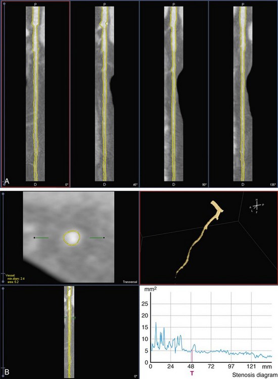
 FIGURE 84-4
Stenosis Quantification
When the contours in the stack of transversal images have been detected, possibly corrected and approved, vessel-related parameters such as the lumen cross-sectional area and diameter are calculated for each individual image (cross-section). Based on this series of measurements, the area function along the vessel and the corresponding minimum and maximum values are determined. The cross-sectional area is directly related to the hemodynamic properties of vessels and is, therefore, expected to be more significant than the vessel diameter measurements. However, because of the historical popularity of projection angiography, the vessel diameter is still commonly used for the quantification of vessel stenosis. We propose using both. Following van Bemmel and colleagues, an average radius of the lumen is derived by comparing the measured area with the area of a circle with a given radius.10 From the actual area function from the beginning to the end of a vessel, a reference area (or diameter function) can be derived, representing to the best of our knowledge the size of the vessel before the obstructions became apparent. This reference function is determined by a repeated linear regression fit of the lumen area as a function of the longitudinal distance.11 The user may flag areas that are suspicious and may cause an erroneous determination of the trend. For example, it is difficult to produce accurate reference contours of a vessel in the vicinity of large bifurcations, or ectatic areas. For such cases, it is justified to remove (flag) these parts from the calculation of the reference function.
Principle
Segmentation Steps
To obtain the centerline and surface model representation of the coronary trees from the CTA data set, a method similar to the approach described earlier can be used. The only difference is that some presegmentation steps are applied before extracting the vessels. Also, the end points for the centerlines within the coronary tree are now automatically found, so that only a single user-defined start point is needed.12
The before-mentioned presegmentation step removes large contrast-filled structures in the image. The removal (or masking) of the large contrast-filled regions, like the heart chambers and the aorta, prevents the WaveProp algorithm from leaking. Starting from a user-defined seed point in the ostium of the coronary tree, the propagation method will result in a complete segmentation of the arteries in the tree. From this user-defined point, the “root” point, the extremities of the coronary tree, called the “leaf points”, can be determined automatically. Next, the centerlines of the coronary tree are detected as described earlier. An example of the outcome of these segmentation steps is presented in Figure 84-5.
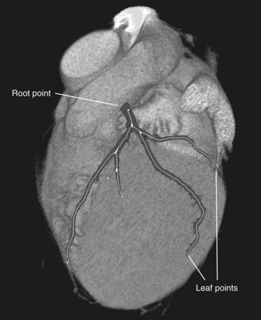
 FIGURE 84-5
Region of Interest
To obtain the optimal angiographic viewing angle for a specific bifurcation, a region of interest for that bifurcation is defined at 10 mm distance from the bifurcation point (Dregion in Fig. 84-6A).
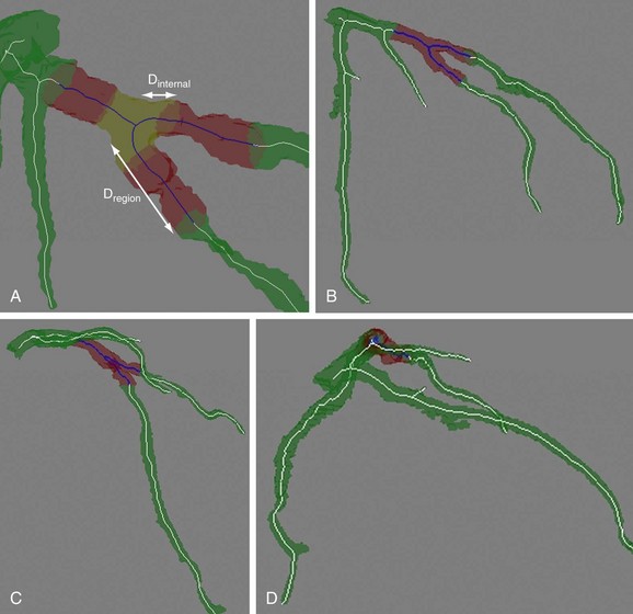
 FIGURE 84-6
Projection Overlap
To determine the projection overlap for a bifurcation, the projected image of only the bifurcation region is calculated first, followed by the calculation of the projection of the remainder of the coronary tree (without the bifurcation). The projection overlap for the bifurcation is defined by the number of pixels that appear in both the projection of the bifurcation and the projection of the whole coronary tree. Figure 84-6 shows examples of the projection overlap of a bifurcation for different angles. To distinguish between the examples a and c, which have similar overlap and foreshortening values, a second overlap measure is defined, which is denoted by the internal overlap. This internal overlap determines the overlap that individual branches of the bifurcation have with each other. For this, the three branches of the bifurcation are separated from each other (see Fig. 84-6A) and the overlap between each branch pair is calculated. The internal overlap for the whole bifurcation is defined by the maximum value of these pair-wise overlap values.
Stay updated, free articles. Join our Telegram channel

Full access? Get Clinical Tree


