1 THREE DIMENSIONAL ANALYSIS OF HEART GEOMETRY AND FUNCTION
Heart System Research Center, The Julius Silver Institute,
Department of Biomedical Engineering,
Technion-Israel Institute of Technology,
Haifa, 32000, Israel
1.1. INTRODUCTION
The heart is an organ that functions by a periodic change of its three dimensional (3D) shape. The pumping function of the heart is characterized by a highly temporally ordered periodic change of the 3D spatial geometry of the heart’s chambers. The instantaneous cardiac shape is an important parameter which reflects on the complex shape-function interactions of the electric, metabolic, neural and mechanical control systems. It determines the blood volume enclosed within its main cavities, namely the left ventricle (LV) and the right ventricle (RV), and couples between the blood pressure and the myocardial strains (e.g., through the Law of Laplace1).
The LV shape changes determine the blood flow to the aorta and consequently the LV blood pressure and the coronary flow. The most evident manifestations of the shape-function relationship may be observed in developed cardiac pathologies2–8 such as fibrous aneurysms, ischemic scars and others; these are usually manifested by the global changes of cardiac shape (e.g., dilatation of the ventricles, thin aneurysmal walls) as well as by abnormal cardiac motion.2,3,5 While these can be based on comparing LV wall thickness and motion only between end-diastole (ED) and end-systole (ES), the temporal sequence of contraction may highlight cardiac pathologies.9,10 Thus, by quantitatively analyzing the heart’s geometry and its temporal changes one can characterize the functional state of the heart and learn to distinguish between normal and abnormal conditions.11
In vivo heart geometry is best defined by imaging. However, in most previous studies are based on two dimensional (2D) data sets and therefore discard the true 3D cardiac geometry which obviously results in considerable errors.9, 12–14 In this chapter we review and assess some available 3D imaging methodologies for the quantitative analysis and assessment of the normal and pathological heart shape-function relationship.
1.2. CARDIAC IMAGING METHODS
1.2.1. Imaging and Visualization
Imaging denotes the art of converting normally unseen phenomena into observable, visual, entities. Unlike visualization, which identifies normally unseen objects by tracers or otherwise, imaging involves reconstructing the physical entity from data sets generated by the imaging technique. As imaging involves visualization, these two terms are commonly interchanged. Here we consider “imaging” in the broad all inclusive sense of this term.
The outstanding progress in computer technology and image processing techniques allows us to address, simulate and analyze the shape-function relationships in the complicated spatio-temporal 3D systems. Of particular importance is the interplay between the visual entity which provides a quantitative understanding of the studied phenomena, and the quantitative information contained within the visual images. The dynamic field, which represents a spatio-temporal behavior of some parameter, can either be mapped directly by the imaging system as with infrared image sequences, or estimated and reconstructed from appropriate measurement data. The latter is the case of the dynamic 3D cardiac wall thickness which is based on edge detection algorithms and geometrical data. Thus, a data processing stage must precede the visualization stage in most cases, with vectorial data providing topological information from critical field points and connecting surfaces and tensorial data providing streamlines and isosurfaces.
This review relates to unravelling of the cardiac shape-function relationships, which are based on three dimensional (3D) imaging techniques. A short review of the presently available imaging modalities will help put this objective in proper perspective.
1.2.2. Imaging Modalities
The oldest procedure of cardiac imaging is, of course, thoracic X-ray, in which the heart is projected as a dark shadow within the rib cage. The interpretation of the image is mainly qualitative in nature. As the attenuation of X-rays by soft tissue is rather low, the contrast is poor and the obtained images indicate only whether the heart is “normal”, or deviates abnormally from the typical normal size.
Contrast agents improve image resolution. Angiography, first reported by Forssman,15 combines catheterization with injection of contrast agents to the heart cavities or coronary vessels, and provides clear images of the coronary tree and fair images of the heart’s cavities. Angiography, the leading method for detecting coronary artery diseases, is an invasive procedure and involves some risk to the patient. Exposure to non-negligible doses of X-ray radiation during angiography may have a small but definite consequence.
Cardiac ultrasonic imaging, i.e., echocardiography, is completely noninvasive and can therefore be used frequently. Moreover, echocardiography can yield dynamic images of cross-sections of the heart and, combined with color Doppler, provides overlay maps of blood flow patterns. These features make echocardiography the most commonly used imaging modality. However, echocardiography has three major disadvantages: (i) imaging is limited to certain viewing windows (i.e., the intercostal spaces) (ii) image quality is typically fair and (iii) image resolution decreases with range and is in the order of 2–3 mm. While transesophageal echocardiography16 overcomes the first limitation, the other two limitations remain.
An exciting and clinically promising ultrasonic technology involves intravascular echography.17 Though invasive in nature, this procedure allows to view the stenotic regions in the coronaries and thus greatly affects the therapeutic procedure.
Radioactive based imaging techniques such as the Gamma-Camera, single photon emission tomography (SPECT) and positron emission tomography (PET) permit the in vivo application of tracer kinetic principles. Tracer amounts of isotope-labelled compounds are administered intravenously or by inhalation, allowing to derive clinically significant temporal or spatial information on the tracer concentration and activity in the tissue. Tracer kinetic models can relate the temporal changes in the tracers’ concentration to metabolic rates, regional myocardial blood flow and oxygen consumption. High temporal resolution of modem PET scanners allows to quantify the relationship between substrate delivery, transmembrane transport and intracellular substrate utilization, and the spatial distribution and heterogeneity of these processes in the normal and diseased myocardium can be mapped and evaluated.18 Unfortunately, the relatively poor spatial resolution of these techniques prohibits relating these functions to the true geometry of the heart. Other sophisticated imaging tools such as computer tomography (CT) and magnetic resonance (MR) are therefore needed when searching for the shape-function relationships in the cardiac muscle.
The introduction of fast CT techniques into cardiology involved shortening the data acquisition time to several milliseconds, and obtaining sequential exposures representing one heart beat. Two techniques are presently available: the digital spatial reconstructor (DSR)19 and the Cine-CT.20 Both techniques provide high spatial resolution images (pixels of about 1 mm in size) with high quality and high temporal resolution. However, these techniques expose the patient to relatively high doses of X-ray radiation and require intravenous injection of contrast material. Furthermore, these techniques typically provide only sets of short axis images taken by “slicing” the long axis of the heart.
Magnetic resonance imaging (MRI), is noninvasive and the magnetic field involved in the measurement does not cause any detrimental effects on the tissue. It can provide images along any arbitrarily selected plane and may provide high quality, high resolution data. Sufficient temporal resolution is obtained either by applying ECG gated acquisition or by using rapid acquisition methods (e.g., echo-planar,21 or spiral imaging22). In addition, MRI can be applied in 3D imaging on the entire volume contouring the heart. It can be used along with contrast materials to depict perfusion maps, and along with MR spectroscopy to provide metabolic information. Moreover, MRI has a unique feature: the ability to noninvasively tag certain regions of the myocardium.23,24 Finally, recent developments in the field involve MR coronary angiography, which may become a revolution in diagnostic catheterization once resolution and motion problems are overcome. MRI is a most effective and versatile imaging tool available today, but high operation costs are still a major factor hindering its wide clinical application in cardiology.
1.3. DATA MANAGEMENT
One can roughly divide the imaging data sets into four major categories:
(i) | Projection type images: Information is obtained from shadows of semi-transparent objects; this is typical of X-ray angiography and some radioactive based imaging techniques. |
(ii) | Multi-slice parallel plane images: This is typical of the tomographic techniques (Figure 1A). |
(iii) | Axially rotated images: Images are typically obtained along planes rotated around the LV long axis, as in apical echocardiography25 (Figure 1B). |
Arbitrarily oriented planes: Cross-sectional images of the heart are obtained along arbitrarily oriented planes. This category is typical of 2D echocardiography, and can also be implemented in MRI, though less frequently than category (ii). Note that in 3D echocardiography the spatial orientation of each plane is known either by using a spark system26 or by applying an iterative matching procedure27 (Figure 1C). |
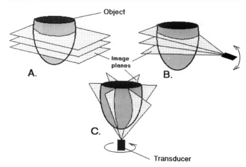
Figure 1. Typical imaging data sets available for 3D computer reconstruction of the heart. (A) Multi-slice parallel plane images. (B) Axially rotated images. (C) Arbitrarily oriented planes.
Another classification of data management relates to stationary (or rather quasistationary) data and dynamic data. The quasistationary data is usually taken at well defined reproducible temporal or spatial end-points in the cardiac cycle. The most common points of reference are the end-diastolic (ED) and end-systolic (ES) states, which are commonly used as reference points to study changes during the entire cardiac cycle and for comparison between different hearts. The dynamic data is taken either continuously, as in the case of tracers, or intermittently during the cycle, thus presenting a finite sequence of images between ES and ED.
Practically all the work reported here relates to the analysis of the stationary and the intermittent-dynamic cardiac data.
1.4. TWO DIMENSIONAL (2D) LEFT VENTRICULAR SHAPE ANALYSES
The first quantitative analysis of the LV geometry is probably due to Woods28 who in 1892 applied the Laplace equation to incised and preserved hearts. In its simplest form the Laplace equation states that:
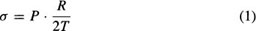
where σ is the stress induced in the myocardial wall, P is the LV cavity blood pressure, T is the wall thickness and R is the LV radius of curvature. As can be concluded from Equation (1), the geometrical factor R/T determines the stress within the myocardium which “resists” contraction. This equation can provide a general explanation why dilated hearts are weaker, as a larger R induces a larger σ and why pathological high pressure results in hypertrophy of the wall, i.e., σ decreases as T increases.
Woods’ quantitative approach gained clinical acceptance29,30 and the curvature/thickness ratio, R/T, was investigated in vitro31 and in vivo32 using angiographic or echocardiographic images, and recently, 3D MRI.
Quantitative assessment of the LV by assuming spherical or ellipsoidal geometries is convenient but insufficient, as the LV radius of curvature varies with location. Gibson and Brown33 suggested a non-dimensional 2D shape index (SI), which can be used to quantify the roundness of the LV shape.
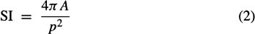
where p is the LV shape perimeter and A is its area. SI equals unity for a perfect circular shape and has values < 1 for elliptic shapes. The advantage here is that this index relates to the entire LV shape and does not rely on regional measurements. However, this index is not directional, and longitudinal and lateral elongation of the LV can yield identical SI value.
A more directional “eccentricity” index (E), was suggested by Fischel et al.:34
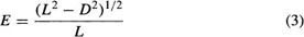
where L is the LV major axis and D is the LV minor axis, both measured from angiographic projection images. Obviously, E = 0 for a perfect sphere and its value increases as the heart becomes more elongated (E = 1 for a straight vertical line).
Azancot et al.35 suggested the application of the Fourier transform to the traced echocardiographic 2D cross-section images of the LV. This approach was adopted by Kass et al.,36 who implemented spectral indices to angiographically obtained contours. They have shown that the shape characteristics of LVs with aortic regurgitation differ significantly from that of normal hearts. A slightly different approach was suggested by Duvernoy et al.37 who have replaced the Fourier transform representation by a Fourier descriptor for closed curves. Their descriptor has the advantage of being insensitive to translation, rotation and scaling of the image.
Marcus et al.38 compared a number of quantitative methods for characterizing LV contraction based on 2D angiographic data and proposed a rather unique curvature dependent approach to the shape analysis. Halmann et al.10 extended this procedure and proposed a dynamic analysis of the LV shape based on the curvature function.
1.5. THREE DIMENSIONAL (3D) SHAPE ANALYSIS
1.5.1. Shape Characterization
The obvious disadvantage of all 2D procedures for characterizing the LV shape is that they discount the 3D geometry of the heart and thus yield erroneous results. However, early attempts to characterize the heart’s 3D geometry have either used geometrical assumptions about the shape to reach conclusions about the shape,39 or were too cumbersome for practical use (e.g., the multi-chart approach by Janicki et al.,40 or the spherical harmonics by Schundy et al.41). With the advancement of new imaging modalities such as Cine-CT and MRI, in vivo data covering the entire heart can be obtained and utilized to investigate the in situ 3D geometry. Typical Cine-CT scans are depicted in Figure 2.
1.5.2. The Geometrical-Cardiogram (GCG)
A novel procedure for describing the spatial geometry of the LV by using a special helical shape descriptor was suggested by Azhari et al.42,43 The procedure assumes that the LV is enclosed within an imaginary cylinder with a diameter larger than the larger diameter of the LV. Moving along a helical path on the cylinder (Figure 3), and measuring the radial distance R from the surface of the cylinder to the endocardial (or epicardial) surface of the LV, yields a function R(ξ) which describes a spatial curve wrapped around the LV shape and can be used to approximate its geometry. It is important to note that the accuracy of this 3D description is inversely proportional to the helical step H0 and the description is exact when H0 → 0.
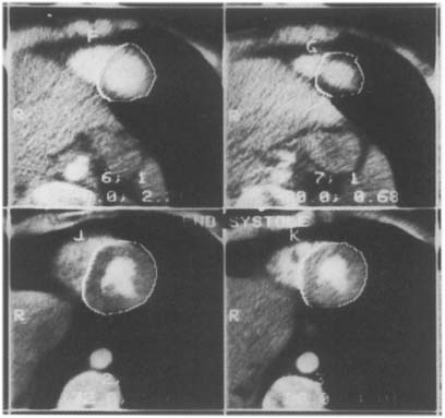
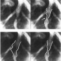
Figure 2. Four typical Cine-CT cross-section images of a human heart. Ten to twelve such cross-sections are commonly required to cover the entire heart with an interslice distance of about 1 cm. Note that the LV epicardial boundary is traced in these images.
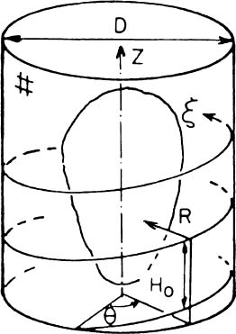
Figure 3. Schematics of the enclosing cylinder and coordinate system utilized to obtain the helical shape descriptor (printed with permission from Azhari et al.42 ©1987 IEEE).
The major advantage of the derived function R(ξ) is that it describes the 3D geometry by a unidimensional vector, and common unidimensional signal processing operators (e.g., filters and transformations) can be readily applied to manipulate the spatial geometry.
Keeping the number of windings needed to reach the base from the apex constant assures that each point along the helix retains its relative height, regardless of the size of the heart. Furthermore, the LV long axis is aligned with the imaginary cylinder axis, and the direction connecting the long axis and the middle of the septal wall is defined as the reference direction from which the helix begins. Thus, each point along R(ξ) retains its relative circumferential position regardless of the size of the heart. Finally the length of the path along R(ξ) is normalized, so it is zero at the apex and 1 at the base and the lateral dimensions are normalized by the length of the LV long axis. (The normalized helical coordinate is denoted as η and the normalized radial coordinate is denoted as ρ.) The ensuing nondimensional helical vector ρ(η) which describes the normalized 3D geometry of the LV, is denoted “geometrical cardiogram” (GCG).43,44
The ability of the GCG to describe the geometrical features of the studied 3D object regardless of the object’s size, is easily demonstrated by applying the GCG to sets of well defined geometries (cylinders, spheres, ellipsoids). Indeed, all the cylinders yield an identical GCG which looks like a step function; the cones yield an identical ramp-like GCG signal, and all spheres and all ellipsoids with the same aspect ratio yield typical GCG signals, regardless of their size.
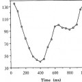
A set of GCG signals obtained for a group of normal human hearts at ED is depicted in Figure 4. The similarity between these “normal” signals under normal conditions suggests that the features of the normal GCG pattern can be characterized quantitatively and, consequently, that GCG signals from abnormal hearts which have a distorted geometry could be identified as significantly different from the normal pattern. This distinction is achieved by utilizing a “shape distortion index” (SDI) which is based on the Karhunen-Loeve Transform (KLT).44
Given a set of N dimensional characteristic pattern vectors  which represent the GCG signals typical to the normal population, it is possible to expand every vector
  from the set by an arbitrary yet complete set of orthonormal basis vectors
  , without loosing any information. However, when only the first K basis functions of the expansion are used, an approximation
  of the expanded vector
  is obtained:
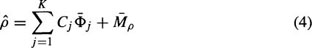
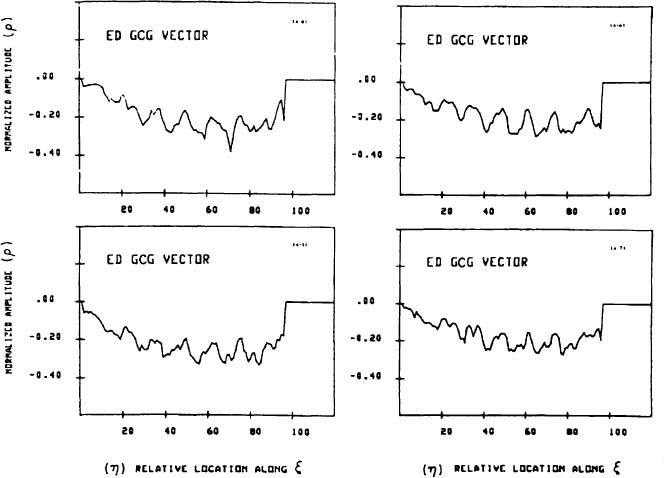
Figure 4. A typical set of GCG signals obtained for four different normal human LV’s at ED (printed with permission from Azhari et al.44 © 1989 IEEE).
 , and
, and  is the mean vector of the set;
  is the expected value operator). The discrepancy between the original vector
  and its approximation
  is evaluated by the mean square error (MSE), which is given by:
The most unique feature of the KLT is that for any number of K terms used in Equation (4), the approximated vector  has the minimal possible MSE. The KLT is optimal in the sense that it compresses the information into uncorrelated basis vectors with a descending degree of importance. Unlike the Fourier and other transforms, the basis vectors
  are not known a priori but are “tailor made” for the studied reference population.
1.5.3. The Shape Distortion Index
The KLT can be utilized to discriminate between normal and pathological hearts based on their 3D geometry.44 This involves obtaining a set of KLT basis functions for the endocardial ED and ES of the reference normal group and for a group of patients with a cardiac disease. The MSE for the abnormal hearts are consistently larger than the MSE for normal hearts. A typical 3D reconstruction of a normal LV and an abnormal one are compared to their KLT reconstructions in Figure 5. Note the much larger discrepancy for the abnormal heart. Optimization yields that the first four ES KLT basis functions have the best discriminatory power.44 The distortion of the pathological heart in comparison to the normal one can be quantified by defining the shape distortion index (SDI):
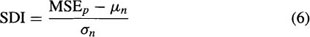
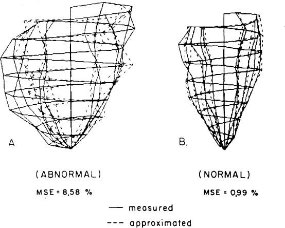
Figure 5. 3D wireframe reconstructions of two human LVs demonstrating the implication of different MSE values. The solid line corresponds to the measured data and the dashed line to its corresponding KLT approximation. (A) Abnormal LV (B) Normal LV. Note the large discrepancy between the measured and approximated shapes in the abnormal case with contrast to the close approximation obtained for the normal LV (printed with permission from Azhari et al.44 © 1989 IEEE).
where MSE is based on the first four ES KLT basis functions for the particular heart under study, μn and σn are, respectively, the average and MSE values obtained for the group of normal hearts. Note that by definition the expected SDI value for normal hearts is zero, and assuming a Gaussian distribution for the SDI values, a heart with an SDI > 3 may be categorically considered abnormal (p < 0.04). The SDI values for the group of abnormal hearts ranged between 8.61 to 17.32,44 indicating that the suggested technique has clinical merit.
The KLT based shape distortion analysis is also useful in localizing regional abnormalities,45 as in hearts with aneurysm. The regional shape deviation from the expected normal shape is determined by evaluating the KLT reconstruction error for each point along the GCG vector. Thus, the GCG obtained by the KLT based shape analysis may not only detect hearts with aneurysm but also locate the aneurysmal regions.
1.5.4. Sorting Pathological Hearts
The ability to distinguish between normal and ischemic hearts by the GCG based shape analysis12 led to investigate the possibility of using the GCG to sort between abnormal hearts with different pathologies.46 As is well known, different geometric distortions may be generated by different pathologies. However, the GCG spectral decomposition may help in sorting the different diseases by determining their geometrical characteristics.
As shown by Azhari et al.,46 the GCG can be expressed analytically by a Fourier-sine series:
where An designates the amplitude of the nth harmonic, and η = 0 corresponds to the apex and η = 1 to the LV base. Since the left hand side of Equation (7) represents a 3D shape, each harmonic on the right hand side must also represent a 3D shape.
Consider the first harmonic. If A1 is not zero, then moving along η from apex to base describes a helical trajectory in space which encloses a football shape (Figure 6A). Mathematically this shape is obtained by rotating a single lobe of a sine function with amplitude A1 around the LV long axis. As the absolute value of A1 is increased, the shape grows in the lateral direction. Decreasing A1 yields a laterally narrower shape, assuming the form of a cigar. Note that due to the definitions of the GCG, an harmonic with A1 < 0 describes a real object, and an harmonic with A1 > 0 describes a “hole” in space with a shape similar to the one described.
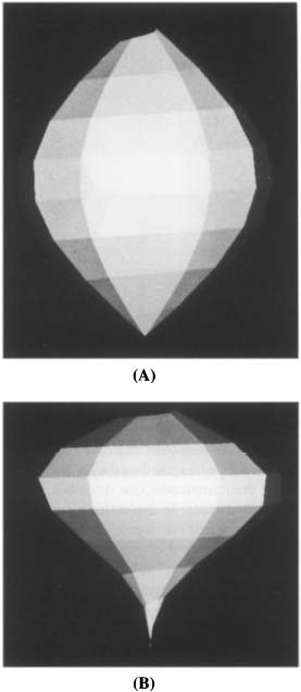
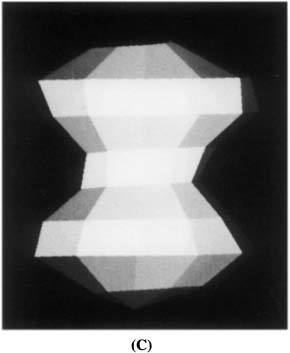
Figure 6. The 3D interpretation of the GCG spectral decomposition. (A) 3D reconstruction of the GCG first harmonic. Note that for A1 < 0, this shape corresponds to a real object while, for A1 > 0, this shape corresponds to a “hole” in space. (B) 3D reconstruction of the GCG first and second harmonics. (C) 3D reconstruction of the GCG first and third harmonics. Note that a different shape is obtained if A3 and A1 differ in signs.
Next, consider the second harmonic. The shape described by this harmonic has two lobes, like two footballs spiked on the LV long axis. As the two lobes differ in the signs of their amplitude, one describes a real object while the other describes a “hole” in space. To depict this geometry we combine it with a real object defined by the first harmonic. The result is a “tear-drop” shape (Figure 6B), which points upward or downward, depending on the sign of A2; in normal hearts the “tear-drop” points upward.
Finally, consider the third harmonic. This harmonic has three lobes, “spiked” along the LV long axis, representing a real part at the top and a real part at the bottom and a “hole” in the center, or vice versa. The results of combining the third and first harmonics are depicted in Figure 6C for the case common to normal human hearts.
The spectral decomposition of the GCG allows to determine the geometrical regularity of the shape. As shown,46 the contribution of each harmonic to the volume enclosed by the LV shape is proportional to the square of its amplitude; higher harmonics correspond to the more complicated features of the studied shape. Consequently, the higher the relative contribution of the lower harmonics to the volume of the studied shape, the more regular it is. The geometrical regularity index (GRM) allows to quantify this feature:
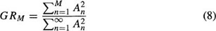
Using the amplitudes of the first three harmonics, i.e., A1, A2 A3 and the geometrical regularity index GRM for M = 8 in Equation (8), suffices to characterize human hearts. The results are depicted in the A3–GR8 parametric space for 10 normal hearts, nine aneurysmal hearts, five with myocardial infarction and three with hypertrophy, in Figure 7
Related posts:
Stay updated, free articles. Join our Telegram channel

Full access? Get Clinical Tree


