, is the current that flows within neurons and across their membranes, and is the quantity of interest in neuroscience. Because the cells are embedded in an electrically conducting medium, the extracellular current—also called the the “return” current—follows a path that depends upon the conductivity profile of the extracellular medium. The return current  is taken to be the product of the local conductivity
  and the electric field intensity
  , i.e., it is ohmic current. The complete current becomes
(1)
Electric current either flows in closed circuits or else, if it starts or stops somewhere, electric charge builds up (or declines) at such locations. This is embedded in the fundamental principle of ‘charge conservation’, the mathematical statement of which is the continuity equation
where  is the charge density. Equations (1) and (2) together with the Maxwell equation that embodies Gauss’s Law,
  , lead to
where the characteristic frequency  . Even for the skull, which is the part of the head with the smallest conductivity,
  is approximately
  Hz. This is orders of magnitude greater than the frequencies of neuronal activity, which are in the range 1–1,000 Hz.
(2)
is the charge density. Equations (1) and (2) together with the Maxwell equation that embodies Gauss’s Law, , lead to(3)
. Even for the skull, which is the part of the head with the smallest conductivity, is approximately Hz. This is orders of magnitude greater than the frequencies of neuronal activity, which are in the range 1–1,000 Hz.2.1 Regions of Constant Conductivity
It requires many thousands of nearby neurons acting in near synchrony to produce a signal strong enough to be detected by EEG or MEG. Since the electrical conductivities of the various compartments of the head are not known in any spatial detail, it is common to assign an average value to the brain, one to the cerebrospinal fluid, one to the skull and one to the scalp.
2.1.1 The Electric Field
In any region of constant conductivity a number of conclusions follow from Eq. (3), where the term  drops out.
drops out.(i)
Away from primary current any electric charge must fall off with time as  .
.
.(ii)
As mentioned above the frequencies of neuronal activity are smaller than  by many orders of magnitude in all the compartments of the head. Hence the term
  is negligible compared to
  in Eq.(3).
by many orders of magnitude in all the compartments of the head. Hence the term is negligible compared to in Eq.(3).(iii)
At the site of primary current charge can persist for the duration of the current, and then falls off as in (i).
(iv)
Electric charge can also appear at the boundary between regions of different conductivity. This will be discussed later.

A further approximation for  will follow after consideration of the magnetic field.
will follow after consideration of the magnetic field.2.1.2 The Magnetic Field
From the Maxwell equation  , which says that there are no magnetic monopoles, it follows that
  can be written as
  , where
  is called the vector potential. This makes use of the vector identity
  .
.
, which says that there are no magnetic monopoles, it follows that can be written as , where is called the vector potential. This makes use of the vector identity .From Faraday’s Law comes the Maxwell equation  , which means that the electric field can be written in terms of the scalar potential
  and the vector potential as
, which means that the electric field can be written in terms of the scalar potential and the vector potential as(5)
The proof follows by taking the curl of both sides of Eq. (5) since  .
.
.Any electric current gives rise to a magnetic field, and this is embodied in the fourth Maxwell equation
(6)
The final term in Eq. (6) is called the Displacement Current, and  is the speed of light. Putting that term there was Maxwell’s great achievement to insure that charge is conserved, as can be checked by taking the divergence of both sides of the equation.
is the speed of light. Putting that term there was Maxwell’s great achievement to insure that charge is conserved, as can be checked by taking the divergence of both sides of the equation.Since the magnetic field arises from the current,  and
and  follow the time dependence of
  . This places an approximate limit on the magnitude of the time derivative terms in Eqs. (5) and (6) since the maximum frequency of the neuronal activity of interest is
  .
.
and follow the time dependence of . This places an approximate limit on the magnitude of the time derivative terms in Eqs. (5) and (6) since the maximum frequency of the neuronal activity of interest is .For Eq. (6) the return current  makes the first term on the right hand side larger than the second term by the ratio
  , which is many orders of magnitude. For Eq. (5) it takes more work to show that the magnitude of
  is negligible compared to
  . After seeing what follows by neglecting that term, one can go back and verify that the neglect was justified. Combining Eq. (4) with
  gives
gives
which represents the quasistatic approximation for the electric potential in any region of constant conductivity.
makes the first term on the right hand side larger than the second term by the ratio , which is many orders of magnitude. For Eq. (5) it takes more work to show that the magnitude of is negligible compared to . After seeing what follows by neglecting that term, one can go back and verify that the neglect was justified. Combining Eq. (4) with gives(7)
The electric potential is that solution of Eq. (7) which satisfies the boundary conditions that the electric potential is continuous and the normal component of the return current is continuous on the boundary separating regions with conductivities  and
and  . While there may be electric charges on the boundary, continuity of the potential assumes there are no electric dipoles. And continuity of the normal component of the return current assumes there is no source of primary current right on the boundary.
and . While there may be electric charges on the boundary, continuity of the potential assumes there are no electric dipoles. And continuity of the normal component of the return current assumes there is no source of primary current right on the boundary.(8)
To verify that Eq. (9) satisfies Eq. (6) (without the displacement current) requires some algebra which is best handled using component notation. It is correct only if the current  is conserved, i.e., it must be the complete current, satisfying
  . Of course the two contributions to
  coming from the primary and return currents can be evaluated separately, but only the sum of the two is physically meaningful. They are designated as
  and
and  .
.
is conserved, i.e., it must be the complete current, satisfying . Of course the two contributions to coming from the primary and return currents can be evaluated separately, but only the sum of the two is physically meaningful. They are designated as and .Equations (7), (8) and (9) together constitute the quasistatic approximation to Maxwell’s equations. An essential property of Maxwell’s equations is that they are linear in the source charges and currents. This means that the solution of the equations, for the electric field and the magnetic field, for the sum of two sources is the sum of the solutions for the individual sources. Naturally this property also holds for the quasistatic approximation to the equations, and will be used throughout the chapter.
3 The Forward Problem
A head model consists of a specification of the geometry and conductivity of the various compartments of the head, e.g., brain, cerebrospinal fluid, skull and scalp. For any assumed primary current distribution  the ‘Forward Problem’ for EEG and MEG solves Eqs. (7) and (8) for the electric potential, and Eq. (9) for the magnetic field on the surface of the head and outside.
the ‘Forward Problem’ for EEG and MEG solves Eqs. (7) and (8) for the electric potential, and Eq. (9) for the magnetic field on the surface of the head and outside.There are other applications of electromagnetic theory to the brain besides EEG and MEG. For example, if one were interested in the effect of current in the brain on MRI, which is called ‘direct neural imaging’, then one would need the magnetic field inside the brain. For a uniform sphere the solution is given in (Heller et al. 2004). In addition, brain stimulation by an external current source (known as Transcranial Magnetic Stimulation (TMS)) makes use of the electric field induced inside the brain.
3.1 A Current Dipole
Suppose that the primary current occupies a quite localized region, e.g., a few millimeters in size. Then for positions  that are not too close to that current the primary current contribution to the integral in Eq. (9), can be approximated as

where
that are not too close to that current the primary current contribution to the integral in Eq. (9), can be approximated as(10)
(11)
This approximation amounts to concentrating all the primary current at a single position, where  is somewhere inside current. One writes
  , where
  is the Dirac delta function.
  is called the current dipole moment. Note that any current whatsoever, no matter how spread out it may be, can be written as a linear combination of current dipoles. Since Maxwell’s equations are linear in the sources, the solution for the fields becomes a linear sum of the solutions for the individual dipoles. In applications to experimental data it is common to represent the source as the sum of a small number of current dipoles.
is somewhere inside current. One writes , where is the Dirac delta function. is called the current dipole moment. Note that any current whatsoever, no matter how spread out it may be, can be written as a linear combination of current dipoles. Since Maxwell’s equations are linear in the sources, the solution for the fields becomes a linear sum of the solutions for the individual dipoles. In applications to experimental data it is common to represent the source as the sum of a small number of current dipoles.3.2 Special Solutions
To solve Eqs. (7), (8) and (9) for the electric potential and the magnetic field for a general head model requires a numerical solution first for  and then for
  since the return current contribution to
  needs
needs  . But for certain special geometries analytic solutions are available, and the most important one is a spherical geometry in which the electrical conductivity
  is assumed to depend only on the distance from the origin. Although the human head is not a sphere it is not vastly different, and one can get a fair approximation to
  and
and  by treating the brain, skull and scalp as concentric spherical regions. This solution is also useful for checking the accuracy of computer programs written for more general geometries.
and then for since the return current contribution to needs . But for certain special geometries analytic solutions are available, and the most important one is a spherical geometry in which the electrical conductivity is assumed to depend only on the distance from the origin. Although the human head is not a sphere it is not vastly different, and one can get a fair approximation to and by treating the brain, skull and scalp as concentric spherical regions. This solution is also useful for checking the accuracy of computer programs written for more general geometries.3.2.1 The Magnetic Field
For the magnetic field outside the head, where there is no electric current, from Eq. (6) (neglecting the time derivative term)  and therefore
  can be obtained as the gradient of a scalar potential, (Bronzan 1971). With
  a function of
  it was shown in (Grynszpan and Geselowitz 1973; Cuffin and Cohen 1977; Ilmoniemi et al. 1985; Sarvas 1987) that the complete magnetic field due to a point current dipole with moment
  at position
  is
is
![$${\mathbf{B}}({\mathbf{r}}) = \frac{{\mu_{0} }}{{4\pi F^{2} }}[F{\mathbf{p}} \times {\mathbf{r}}_{{\mathbf{0}}} - ({\mathbf{p}} \times {\mathbf{r}}_{{\mathbf{0}}} \cdot {\mathbf{r}})\nabla F]$$](/wp-content/uploads/2016/04/A272390_1_En_3_Chapter_Equ12.gif)
where
and

Written in this form Eq. (12) is called the ‘Sarvas formula’ (Sarvas 1987). Note that it is completely independent of the conductivity function, provided that it depends only on the radial distance from the origin!
and therefore can be obtained as the gradient of a scalar potential, (Bronzan 1971). With a function of it was shown in (Grynszpan and Geselowitz 1973; Cuffin and Cohen 1977; Ilmoniemi et al. 1985; Sarvas 1987) that the complete magnetic field due to a point current dipole with moment at position is(12)
(13)
(14)
Another consequence of considerable importance can be read off Eq. (12). If the dipole moment  points in the same radial direction as its position
  , then
  , and hence there is no magnetic field outside the head. Such a ‘radial dipole’ is the simplest example of what is called a “magnetically silent source”, i.e., an electric current that produces no magnetic field outside the head. A radial dipole does produce a non-zero magnetic field inside the head, however (Heller et al. 2004).
points in the same radial direction as its position , then , and hence there is no magnetic field outside the head. Such a ‘radial dipole’ is the simplest example of what is called a “magnetically silent source”, i.e., an electric current that produces no magnetic field outside the head. A radial dipole does produce a non-zero magnetic field inside the head, however (Heller et al. 2004).The existence of silent sources poses a difficulty for the Inverse Problem, which is discussed in Sect. 4. It consists of trying to deduce the electric currents in the brain that produce an experimentally observed magnetic field and/or electric potential. While an actual current dipole might have both radial and tangential components only the tangential component can be determined. Even though the head is not a sphere a considerable remnant of this uncertainty persists in a realistic head model.
3.2.2 The Electric Potential
Unlike the magnetic field case, the electric potential in a spherical geometry does depend on the values of the conductivity in each concentric region, (Rush and Driscoll 1969). For a uniform sphere an analytic formula for the potential  due to a current dipole moment
  located at position
  is given in (Heller and van Hulsteyn 1992):
![$$\begin{array}{*{20}c} {V({\mathbf{r}}) = {\mathbf{p}} \cdot \nabla_{1} H({\mathbf{r}},{\mathbf{r}}_{1} )} \\ {H({\mathbf{r}},{\mathbf{r}}_{1} ) = \frac{1}{4\pi \sigma }\left[ {\frac{2}{{|{\mathbf{r}} - {\mathbf{r}}_{1} |}} - \frac{1}{r}\ln \frac{{{\mathbf{r}} \cdot ({\mathbf{r}} - {\mathbf{r}}_{1} ) + r|{\mathbf{r}} - {\mathbf{r}}_{1} |}}{{2r^{2} }}} \right],(r \ge R,r_{1} \le R)} \\ \end{array}$$](/wp-content/uploads/2016/04/A272390_1_En_3_Chapter_Equ15.gif)
where  is radius of the sphere. This difference between the two modalities MEG and EEG, has the following consequence. Suppose the skull, which has a small electrical conductivity, did not conduct current at all. Then there would be no such thing as EEG because no current, and hence no electric field or potential, would be present at the scalp. The magnetic field, on the other hand, penetrates through regions that have no electrical conductivity.
due to a current dipole moment located at position is given in (Heller and van Hulsteyn 1992):(15)
is radius of the sphere. This difference between the two modalities MEG and EEG, has the following consequence. Suppose the skull, which has a small electrical conductivity, did not conduct current at all. Then there would be no such thing as EEG because no current, and hence no electric field or potential, would be present at the scalp. The magnetic field, on the other hand, penetrates through regions that have no electrical conductivity.3.3 Realistic Head Models
We now discuss how to solve for the electric potential and the magnetic field in a realistic head model obtained from magnetic resonance imaging of an actual head, together with the assumed conductivity values for the various compartments of the head.
3.3.1 The Electric Potential
The most useful method to solve Eq. (7) for the electric potential in a realistic head model, subject to the boundary conditions in Eq. (8), was given by (Geselowitz 1967). It consists of converting the linear partial differential Eq. (7) to a linear integral equation on the boundaries that separate regions of different conductivity. As shown below, it has the advantage that the boundary conditions are built right in! The starting point is an identity

which is then integrated throughout the entire volume of the head model, one conductivity region at a time. Vector  is a position anywhere inside the head model. On the left side of Eq. (16) one makes use of the divergence theorem, which says that the integral of the divergence of a vector throughout a volume
  is equal to the integral over the surface
  of that volume of the component of the vector along the direction of the outward pointing normal vector. On the right hand side of Eq. (16) one can make use of Eq. (7) to replace
  . Also,
  .
.
(16)
is a position anywhere inside the head model. On the left side of Eq. (16) one makes use of the divergence theorem, which says that the integral of the divergence of a vector throughout a volume is equal to the integral over the surface of that volume of the component of the vector along the direction of the outward pointing normal vector. On the right hand side of Eq. (16) one can make use of Eq. (7) to replace . Also, .Figure 1 shows the notation for the case of three regions, brain, skull, and scalp. The normal vector on each surface is chosen to point outward from that region. It is straightforward to apply Eq. (16) to the innermost (brain) region with volume  , surface
  , and conductivity
  (see Fig. 1). Multiplying Eq. (16) by
  and integrating it throughout region 1 yields
![$$\begin{gathered} \int\limits_{{S_{1} }} {dS_{1}^{{\prime }} {\mathbf{n(r^{\prime})}}} \cdot \left( {\sigma_{1}^{{\prime }} V_{1} ({\mathbf{r^{\prime}}})\nabla^{\prime}\frac{1}{{|{\mathbf{r}} - {\mathbf{r^{\prime}}}|}} - \frac{1}{{|{\mathbf{r}} - {\mathbf{r^{\prime}}}|}}\sigma_{1}^{{\prime }} \nabla_{1}^{{\prime }} V_{1} ({\mathbf{r^{\prime}}})} \right) \hfill \\ = - \int\limits_{{V_{1} }} {d^{3} r^{\prime}\big[4\pi \sigma_{1}^{{\prime }} V({\mathbf{r^{\prime}}})\delta ({\mathbf{r}} - {\mathbf{r^{\prime}}})} + \frac{1}{{|{\mathbf{r}} - {\mathbf{r^{\prime}}}|}}\nabla^{\prime} \cdot {\mathbf{J}}^{p} ({\mathbf{r^{\prime})}}\big] \hfill \\ \end{gathered}$$](/wp-content/uploads/2016/04/A272390_1_En_3_Chapter_Equ17.gif)
, surface , and conductivity (see Fig. 1). Multiplying Eq. (16) by and integrating it throughout region 1 yields(17)
Fig. 1
A schematic diagram showing three head regions with their respective volumes  , surfaces,
  , and normal vectors
  . In the literature the conductivities of the respective regions are called
  , and a second set of labels, designated
  is introduced for notational reasons. They are related as follows.
  ;
;  ; and
; and  , being the conductivity of the space surrounding the head, is zero
, surfaces, , and normal vectors . In the literature the conductivities of the respective regions are called , and a second set of labels, designated is introduced for notational reasons. They are related as follows. ; ; and , being the conductivity of the space surrounding the head, is zeroIn this equation the normal vector  points outward from the region with conductivity
  . Furthermore, the quantities
  and
and  are the values of those quantities as
  is approached from the interior of volume
  .
.
points outward from the region with conductivity . Furthermore, the quantities and are the values of those quantities as is approached from the interior of volume .When Eq. (16) is integrated throughout region  with conductivity
  , there are two surfaces that contribute to the left side of the equation,
  and
and  . The contribution from surface
  looks just like the left side of Eq. (17) with the subscript 1 replaced everywhere with 2. But because we have already chosen the normal vector on
  to point outward from region 1, which makes it inward pointing to region 2, the contribution of
  to the left side of the equation requires an overall minus sign.
with conductivity , there are two surfaces that contribute to the left side of the equation, and . The contribution from surface looks just like the left side of Eq. (17) with the subscript 1 replaced everywhere with 2. But because we have already chosen the normal vector on to point outward from region 1, which makes it inward pointing to region 2, the contribution of to the left side of the equation requires an overall minus sign.When the equations for conductivity regions 1 and 2 are summed over the contribution from  contains
  and
and  . Applying the boundary conditions Eq. (8) on
  ,
,  and
and  . This confirms the statement earlier that the integral equation has the advantage over the differential equation that the boundary conditions are built in.
contains and . Applying the boundary conditions Eq. (8) on , and . This confirms the statement earlier that the integral equation has the advantage over the differential equation that the boundary conditions are built in.After integrating Eq. (16) over the complete volume of the head the result is, (Geselowitz 1967)
(18)
In Eq. (18) the position  is anywhere in the volume, and
  is the value of the conductivity in the head compartment containing that position. The final integral on the right side is obtained by once again using the divergence theorem on
  and noting that there is no contribution from the surface integral on the surface of the head because there is no primary current there.
is anywhere in the volume, and is the value of the conductivity in the head compartment containing that position. The final integral on the right side is obtained by once again using the divergence theorem on and noting that there is no contribution from the surface integral on the surface of the head because there is no primary current there.Equation (18) determines the value of the potentlal at position  only if one already knows its values on all the surfaces of discontinuity of the conductivity. To obtain those values let the point
  approach a position
  on one of the surfaces,
  . Care must be taken because the denominator of the surface integral vanishes there.
only if one already knows its values on all the surfaces of discontinuity of the conductivity. To obtain those values let the point approach a position on one of the surfaces, . Care must be taken because the denominator of the surface integral vanishes there.There is a geometric meaning of the integrand which reveals the problem and points to the solution. Apart from the function  the rest of the integrand in the surface integral in Eq. (18) is just the element of solid angle
  subtended at the position
  by an element of surface area
  at position
  , i.e.,
the rest of the integrand in the surface integral in Eq. (18) is just the element of solid angle subtended at the position by an element of surface area at position , i.e.,(19)
Now the total solid angle subtended at any position  inside a closed surface (with outward pointing normal) is
  ; if
; if  is outside the surface the total is zero, and if
  is on the surface the total is
  . It is a discontinuous function. It is equally true with any function
  in Eq. (18) that the limit of the surface integral as
  approaches a position
  on the surface is not equal to the value of the integral with
  ; there is an extra term (Vladimirov 1971)
inside a closed surface (with outward pointing normal) is ; if is outside the surface the total is zero, and if is on the surface the total is . It is a discontinuous function. It is equally true with any function in Eq. (18) that the limit of the surface integral as approaches a position on the surface is not equal to the value of the integral with ; there is an extra term (Vladimirov 1971)(20)
For the final step, in Eq. (18) let  approach
  from the
  side, and replace the limit of the surface integral on surface
  according to Eq. (20). Then there will be an additional term on the right side of
  . When this term is brought over to the left side of the equation, which consists of
  , and the two terms combined, the result is, (Sarvas 1987)
approach from the side, and replace the limit of the surface integral on surface according to Eq. (20). Then there will be an additional term on the right side of . When this term is brought over to the left side of the equation, which consists of , and the two terms combined, the result is, (Sarvas 1987)(21)
The reader can check that it does not matter if the point  approaches
  from the
  side or the
  side; Eq. (21) results either way. [Recall that the normal vector on the
  side has the opposite sign.]
approaches from the side or the side; Eq. (21) results either way. [Recall that the normal vector on the side has the opposite sign.]Equation (21) is a set of coupled linear integral equations for the electric potential, one equation for each surface. A standard method for numerically solving Eq. (21) for the electric potential on those surfaces is to approximate each surface separating different conductivity regions by a set of small triangles, noting that there is an analytic formula for the solid angle subtended by a triangle at an arbitrary position, (van Oosterom and Strackee 1983). Some treatments choose the vertices of the triangles as the locations for evaluating the potential, and some choose the centers of the triangles. See, for example, (Schlitt et al. 1995). When this is done the continuous integral equation is replaced by a set of ordinary coupled linear algebraic equations, which are solved by standard matrix techniques. Figure 2 shows a mesh of triangles on the brain-skull interface, and the outlines of the skull-scalp interface and the scalp-air interface, used for solving Eq. (21).
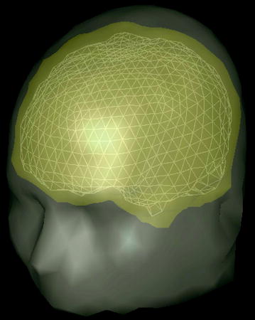
Fig. 2
A mesh of triangles on the brain-skull interface used to numerically solve Eq. (21) for the electric potential. There are similar meshes on the skull-scalp interface and the scalp-air interface, which are not shown. The values of the potential at every triangle vertex are the unknowns being solved for, given an assumed primary current
When doing this it is important to make sure numerically that the total solid angle subtended by all the triangles on a given surface at an interior point is  , and zero at an exterior point. And if the point in question is on one of those triangles the total is
  . Consequently, since a flat triangle subtends zero solid angle at any point on itself, all the other triangles on that same surface must subtend a total of
  at any point located on a triangle.
, and zero at an exterior point. And if the point in question is on one of those triangles the total is . Consequently, since a flat triangle subtends zero solid angle at any point on itself, all the other triangles on that same surface must subtend a total of at any point located on a triangle.As mentioned above, once the potential has been found on the surfaces of discontinuity, it can then be evaluated at any other position using Eq. (18).
3.3.2 The Magnetic Field
The starting point for evaluating the magnetic field in a realistic head model is Eq. (9), the Biot-Savart Law. For the primary current contribution simply insert  into that equation,
where V is the complete volume of the head.
into that equation,(22)
For the return current one must have already solved for electric potential  . Since
  , its contribution to the magnetic field is
 Decoding and Brain Machine Interfaces Based on Electromagnetic Oscillatory Activities: A Challenge for MEG
Neuroscience: A New Frontier for Magnetoencephalography?
Decoding and Brain Machine Interfaces Based on Electromagnetic Oscillatory Activities: A Challenge for MEG
Neuroscience: A New Frontier for Magnetoencephalography?
 Integration
 Imaged Pathways of Stuttering
 Current Imaging with Ultra-Low-Field NMR Techniques
 Concurrent EEG and fMRI Intrinsic Networks


. Since , its contribution to the magnetic field is(23)
Related posts:
Decoding and Brain Machine Interfaces Based on Electromagnetic Oscillatory Activities: A Challenge for MEG
Neuroscience: A New Frontier for Magnetoencephalography?
Integration
Imaged Pathways of Stuttering
Stay updated, free articles. Join our Telegram channel
Full access? Get Clinical Tree
