smaller MR scanners employ resistive coils, others are constructed over permanent, ferromagnetic magnets, but none of these can produce fields as strong and stable as those based on superconducting coils. A main reason to apply strong fields is that the signal-to-noise ratio in the radio signals used to construct the MR image thereby improves.
A whole body MR scanner is voluminous and expensive and not needed for many purposes. Smaller scanners just big enough to accommodate an arm, a leg, or a head have therefore also been developed.
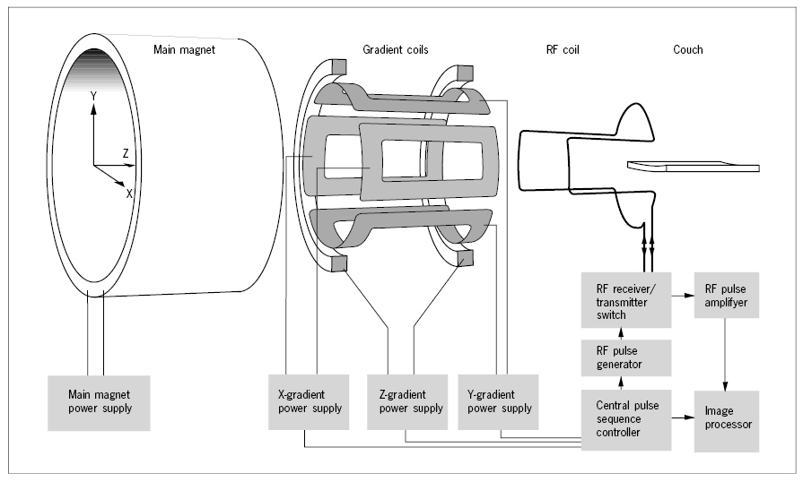
Inside the bore of the magnet are installed three sets of coils used for production of magnetic field gradients, one in the direction of the main field (the Z-axis) and two perpendicular to this (the X- and Y-axis). The gradient field strengths over the entire patient are less than 1% of the main field strength and can be rapidly varied in time. Inside the gradient coil assembly is mounted a radiofrequency (RF) transmitter/receiver coil. For some applications, a small, separate receiver coil, molded to the surface contour of the body part examined, denoted a surface coil, is placed directly on the surface of the body. This improves the signal-to-noise ratio and the resolution in the final image, but limits the volume that can be examined.
The patient is finally installed on a couch centrally in the bore. A pulse sequence controller operates the gradient coil power supplies and the transmitter-receiver switch of the RF coil through the complex sequences used for the various MR imaging modes. The received RF signals are analyzed by Fourier transformation and spatially decoded in the image processor to be displayed as an image, which is a map of the amplitude of RF signals emitted from small volume elements, voxels, in an imaginary slice of the patient.
Proton Magnetization
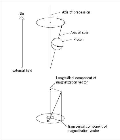
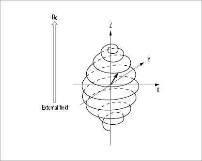
When a proton is exposed to a steady external magnetic field, a force will act on its magnetic dipole moment so as to orient it parallel with the external field, but, due to the spin, it does not swing in as a compass needle would do. Instead it performs a maintained circular movement, called precession, in which its own axis of spin rotates at an angle around another axis that is parallel with the external field, much like a toy spinning top in the gravitational field (Figure 30). The magnetic dipole moment of the precessing proton has a magnitude and a direction and may therefore conveniently be expressed by a vector. This vector may be resolved in one component aligned with the axis of precession, “the longitudinal component”, and a second component, oriented perpendicular to the external field and rotating with the frequency of precession, the “transverse component” (Figure 30).
The frequency of precession, the Larmor frequency, is linearly related to the strength of the external field as expressed by the Larmor equation. The precessional frequency of protons is 42.58 MHz T−1, a constant denoted the gyromagnetic ratio (γ) of the proton (hydrogen). The Larmor frequency is actually not exactly the same for all protons, but differs by a few ppm depending on the chemical bonds they have established. Thus, the Larmor frequency of protons in water and in aliphatic fatty acid chains differs by about 3 ppm (∼130 Hz) in a 1 T field. Such differences are designated chemical shifts. The chemical shifts may cause positional shifts of fat relative to water along the direction of the frequency encoding gradient in some imaging sequences.
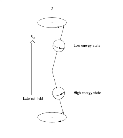
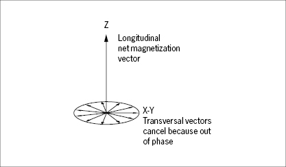
Exposed to the external field, the spin of the proton may be at one of two discrete energy levels, according to principles of quantum mechanics, not to be elaborated here. At the low spin-energy level the longitudinal component of the magnetic vector points in the same direction as the external field, at the high energy level it points in the opposite direction (Figure 31). The fractional distribution of protons between these two states depends on the temperature and the strength of the external field. Even at the high field strengths applied in diagnostic imaging (0.1–2 T), the net magnetization of protons at 37° C is weak with only a small surplus of protons (a few ppm in a 1 T field) being at the low spin-energy level. The net magnetization may, just as the magnetic dipole moment of the individual protons, conveniently be described by a vector (Figure 32). It is important to note that this net magnetization vector represents the statistical equilibrium of a huge population of protons which are constantly influenced by thermal (Brownian) motion, and shifting between the two spin-energy levels. This equilibrium net magnetization vector is aligned parallel (longitudinal) to the external field. The transversal, rotating vectors of the individual protons cancel out because they are out of phase in the equilibrium state.
Resonance
When a body part/tissue has been installed in the strong, steady and uniform field of the MR scanner, the equilibrium state, represented by the net magnetization vector becomes established within seconds. This equilibrium may be disturbed and shifted by a pulse of electromagnetic waves (photons) at the Larmor frequency of the protons (42.58 MHz in a 1 T field) entering perpendicular to the main field. This frequency is within the radiofrequency (RF) region of the electromagnetic wave spectrum (Figure 1). Only RF waves of exactly this frequency will transfer energy by resonance to the precessing protons. In principle, a bar magnet oriented perpendicular to the main field and rotating at 42.58 × 10⁶ revolutions per second would do the same job. This transfer of energy by resonance has two effects on the precessing protons.
Firstly, protons at the low spin-energy level, having absorbed the energy of a RF photon, shift to the high energy state accompanied by a shift in the direction of their magnetic dipole moments. Accordingly, the magnitude of the longitudinal net magnetization vector decreases as more and more protons shift to the high energy state. At a certain RF energy input the longitudinal vector disappears. By further input of RF energy a surplus of protons is lifted to the high spin-energy state whereby the longitudinal vector reappears, but now in the opposite direction.
The second effect of the RF pulse is to force the protons into coherent (“in phase” or “synchronous”) precession. This is manifested by the appearance of a transverse net magnetization vector that rotates with the Larmor frequency.
The net magnetization vector is at any given time the resultant of the longitudinal and transverse magnetization vectors. Thus, with an increasing RF energy input, the longitudinal vector decreases and the transverse vector grows. The net magnetization vector is therefore tilted more and more towards the transverse orientation while rotating at the Larmor frequency (Figure 33). The angle between the direction of the main field and the net magnetization vector is denoted the flip angle. An RF pulse delivering just enough energy to tilt (‘flip’) the net magnetization vector into the transverse orientation is called a 90° pulse. An RF pulse twice this magnitude will cause the reappearance of the longitudinal vector, but in the opposite direction, relative to the main field. Such a pulse is called a 180° pulse and the protons are said to be saturated. RF energy inputs between a 90° and a 180° pulse are said to produce partial saturation. The duration of the excitatory RF pulses used in MR imaging is in the order of a few milliseconds, to give an idea of the timescale.
Relaxation
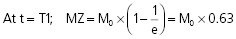
When the RF pulse is turned off, the excited protons return over a period of time to the initial equilibrium state. This process is called relaxation. Now, importantly, the recovery of longitudinal magnetization and the decay of transversal magnetization follow different and independent time courses, both according to simple exponential functions, but with different time constants, denoted T1 for the recovery of longitudinal magnetization, and T2 for the decay of transversal magnetization. T1 is the time at which the longitudinal magnetization has recovered 63% of its equilibrium magnitude. T2 is the time taken for the induced transversal magnetization to decay by 63% (to 37%) of its maximum strength (Figure 34). The two relaxation processes reflect two types of interactions between the precessing protons and their surroundings.
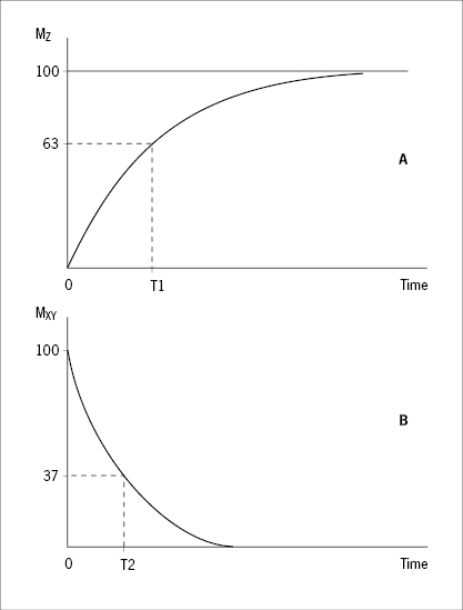
- The exponential recovery of the longitudinal net magnetization vector (MZ) after termination of a 90° RF pulse at time 0.
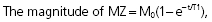
where M0 is the magnitude of the net magnetization vector at equilibrium. T1 is the time constant of the recovery process.
- The exponential decay of the transversal, rotating net magnetization vector (MXY) after termination of a 90° RF pulse at time 0.
The magnitude of MXY as a function of time (t) is given by:
where T2 is the time constant of the decay process.
Recovery of longitudinal magnetization implies loss of energy whereby those protons that were lifted to the high spin-energy state by the RF pulse give up this energy and fall back. This loss of energy is largely of thermal nature with a molecular basis in random collisions with surrounding molecules, collectively called “the lattice”. The longitudinal relaxation process is therefore, according to its nature referred to as the “thermal relaxation time” or the “spin-lattice relaxation time”.
Decay of transverse magnetization implies loss of phase coherence among the precessing protons. This process has its origin in mutual magnetic interactions between the protons, and between the protons and local field inhomogeneities, for example due to the presence of other atoms with magnetic dipole moments and protons precessing at other frequencies due to chemical shifts or due to inhomogeneities/instabilities in the external field. Because interaction between nuclei with different spins is a major contributor to the transversal relaxation process, this is often referred to as the “spin–spin relaxation time”. In pure liquids, characterized by mobile molecules, intrinsic and local field variations are rapidly fluctuating and tend to average out. In solids, molecules are more fixed and local intrinsic field inhomogeneities therefore more permanent, causing protons to systematically dephase. Therefore T2 tends to be short (milliseconds) in solids and long (seconds) in liquids.
T1 will always be longer than T2, but, especially in liquids, they may approach the same value. Tissues may, simplified, be regarded as complex mixtures of solids, solutes in solvent (water) and lipids which at body temperature are somewhere in between solid and liquid. Water and the fatty acid chains of lipids are by far the dominating contributors to the proton MR signals utilized in diagnostic imaging. The other elements may be regarded as elements in a complex “lattice” which shapes the thermal relaxation, expressed by T1, and which creates the local (intrinsic) field inhomogeneities which shape the spin–spin relaxation, expressed by T2. T1 and T2 of a given tissue therefore become sort of averages. Increasing the field strength always increases T1 while T2, in some tissues is largely unaffected, and in others increasing. Actual figures for T1 in a 1 T field varies between different soft tissues from about 200 msec in fatty tissue to about 800 msec in gray matter of the brain. For comparison T1 of pure water is about 2500 msec and about 2000 msec in cerebrospinal fluid (CSF). T2 similarly varies from about 40 msec in liver and muscle to about 90 msec in pure fat and white matter of the brain and about 300 msec in CSF. The chemical shift (∼3 ppm) between protons of water and protons of fatty acids causes especially rapid decay of transverse magnetization in tissues where fat and “watery” tissue is intimately mixed, for example in bone marrow. Dense bone contains too few mobile protons to yield detectable MR signals in diagnostic imaging.
The concentration of protons, detectable by MR imaging in a tissue is denoted the proton spin density or just “proton density” the latter term ignoring that some protons contribute little or nothing to the signal. MR imaging is directed at detection and visualization of differences in spin density and parameters such as T1 and T2 between different tissues and fluids within the body (Figure 35), denoted proton spin density, T1-, and T2 weighted imaging.
Stay updated, free articles. Join our Telegram channel

Full access? Get Clinical Tree


