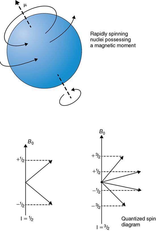
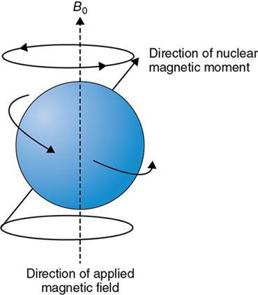
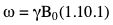
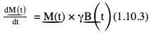
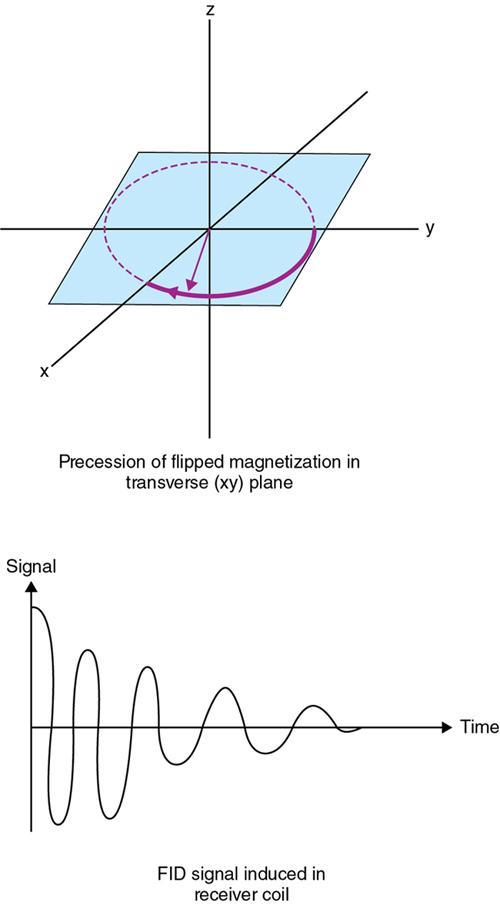
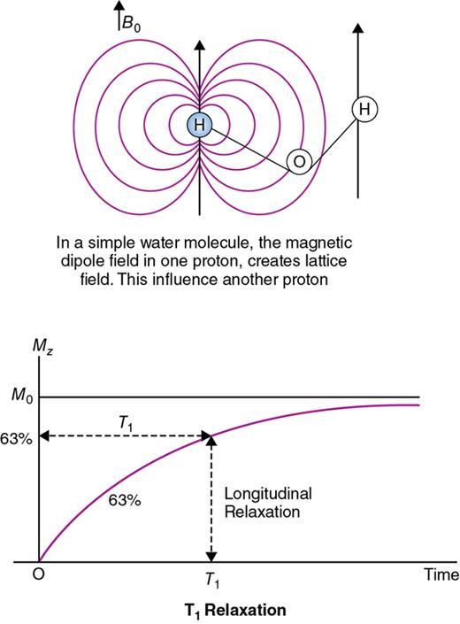
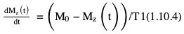
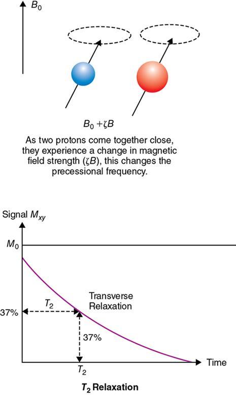
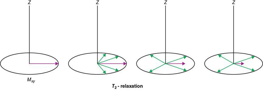
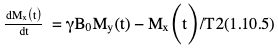
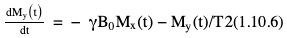
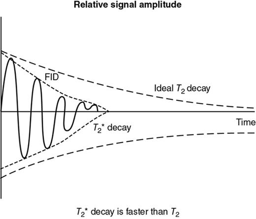
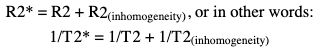
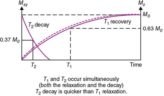
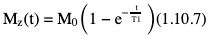
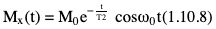
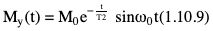
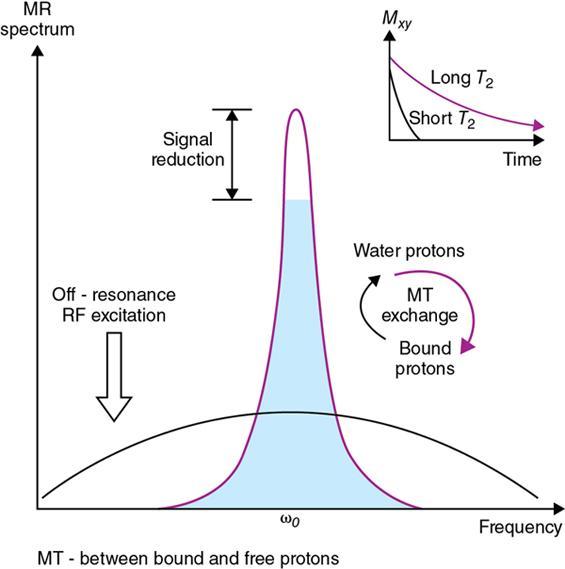
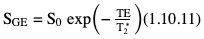
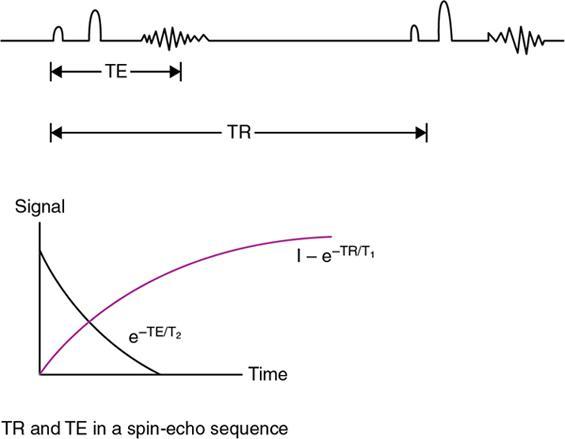
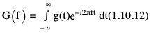
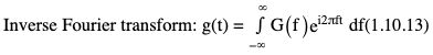
Rupsa Bhattacharjee, Prashant Nair, Jaladhar Neelavalli, Indrajit Saha It was in 1976–77, the first cross-sectional images of the human body were produced using magnetic resonance imaging (MRI). Since then the technology and its clinical applications have evolved and grown exponentially, where today MRI is an indispensable tool in diagnostic imaging. The journey, however, from the discovery of the underlying physical principles to human imaging took a much longer path of evolution. Magnetic resonance imaging is rooted in a much older and rich field called nuclear magnetic resonance or NMR. Two essential properties of the nuclei that are responsible for NMR phenomenon are the spin angular momentum and the magnetic moment. The phenomenon of nuclear magnetic resonance, which makes NMR/MRI possible, was first predicted in 1936 by C.J. Gorter and was later experimentally demonstrated in 1938 by I. I. Rabi, for which he won the Nobel prize in 1944. The experiments showed that a beam of nuclei in a vacuum chamber, subjected to uniform external magnetic field were measurably influenced by radio frequency energy at a characteristic (resonance) frequency. Eight years later, this phenomenon was demonstrated outside of a vacuum chamber, in bulk materials (solids and liquids), by Felix Bloch’s group, and Edward M. Purcell’s group, independently in 1946. These works also laid the foundational understanding of the nuclear spin relaxation mechanisms along with the corresponding mathematical description – often referred to as Bloch Equations. For this work, both Bloch and Purcell received the Nobel Prize for physics in 1952. Until 1950, the phenomenon of NMR was primarily used by physicists to investigate the structure of different atoms. It was generally assumed that different nuclei within a molecule experienced the same uniform magnetic field. However, experiments by Warren Proctor and Fu Chun Yu in 1950, where they observed two separate resonance frequencies for N14 in ammonium nitrate, lead to the postulation that local chemical environment within a molecule can influence the resonance frequency of the nucleus – known today as the chemical shift effect. The following year (1951), Martin Packard, James Arnold and Srinivas Dharmatti showed that hydrogen protons in ethanol (CH3CH2OH) had three distinct resonance frequencies, each corresponding to the CH3, CH2 and OH groups, with the relative amplitudes of their signal being proportional to the number of hydrogen protons. This opened up an entirely new field of chemical and structural analysis of molecules using NMR spectroscopy. Even today, NMR spectroscopy in 1, 2 and 3 dimensions continues to be an active area of research in chemistry and biochemistry, for investigating structure, properties and dynamic interactions of complex biomolecules. It was the work of a few such NMR spectroscopists, which played an important role in the early development of MRI. Since the experiments of Bloch and Purcell in 1946, it took nearly an additional 3 decades for realizing the clinical and imaging applications of NMR and clinicians too played an important role in this. In 1971, Ray Damadian, a medical doctor, discovered that the NMR relaxation parameters of ex vivo normal and cancerous tissue were significantly different and hence may form the basis for non-invasive and early diagnosis. This was still not imaging. A couple of years later, Paul Lauterbur, already a well-known chemistry professor by then, in the field of C13 NMR, published the first proof of concept for imaging using NMR. He used linear field gradients along with the uniform static magnetic field, to make the resonance frequency a function of space, and using that to spatially map the distribution of spins. He successfully used this to show 2D cross-sectional images of two test tubes using multiple projections method, similar to the one used in computed tomography imaging (CT). The use of linear magnetic field gradients to encode spatial location, remains the basis for modern clinical use of MRI today. With the evidence of clinically useful contrast and of the potential to do non-invasive imaging using NMR, many research groups and medical equipment companies across the world focussed their efforts and investment in this field in late 1970s and early 1980s. This was especially a fertile period when several new techniques, quite a few being adapted from NMR methods, for imaging were developed to bring the technology closer to clinical viability. Among them, efforts of John Mallard’s group in University of Aberdeen, Richard Ernst’s group at ETH Zurich and Sir Peter Mansfield’s group in Univ. of Nottingham were especially instrumental in developing time-efficient imaging techniques that brought NMR imaging closer to clinical application. A notable mention is the 3D Fourier Transform-based method proposed by Richard Ernst, Dieter Welti and Anil Kumar in 1975, which is used in almost all clinical imaging today. In parallel, this period of 1970s and 1980s also sparked the development of whole-body scanners. One of the first patients scanned on a whole body scanner (Mark-1) was a carcinoma of the oesophagus at University of Aberdeen, UK, in August 1980. A 2D Fourier Transform-based technique called “spin-warp” imaging was used and the images showed metastasis in the spine and secondary lesions in the liver, which were not suspected. These were later confirmed by nuclear medicine scans. A notable aspect in this period was the drop of the word “Nuclear” from NMR and adoption of the “Imaging” term, to name the new modality as magnetic resonance imaging or MRI. This was mainly to avoid the false connotation of harmful nuclear radiation associated with the term “Nuclear.” The first clinical installation of an MRI scanner after FDA clearance in the United States occurred in 1984 and since then the role of MRI in clinical diagnostic imaging grew leaps and bounds – largely due to the unparalleled soft-tissue contrast and the wide range of tools it provided to probe physiology and pathology non-invasively. One of the key factors that enabled rapid growth of NMR and later of MRI was technology development that happened in parallel in other sectors like computing, semiconductor electronics and superconductivity. Development of high-speed computing, miniaturized electronics and cheaper electronic storage allowed for better system hardware and calibration which in turn enabled production and analysis of larger amounts of imaging data. This, along with better imaging acquisition techniques made 2D and 3D imaging possible in clinically acceptable scan times. India was one of the earliest adopters of the new imaging modality MRI. Clinical magnetic resonance imaging in India started as early as 1986 with the installation of a 1.5 T superconducting magnet at Institute of Nuclear Medicine & Allied Sciences (INMAS), New Delhi. This was made possible by the vision and persistent efforts of Major General Dr. N. Lakshmipathy, who became aware of MRI in 1982 when Dr. R. E. Steiner presented in vivo images of human anatomy during his visit at INMAS. Almost in parallel, Dr. Viral Shah had started his efforts to import an MRI system in private clinical practice in Bombay. His efforts successfully lead to the first installation of an MRI system in a private hospital – Breach Candy hospital in Mumbai and since then, there has been a steady growth of clinical use of MRI in India. As we know within atoms there are fundamental particles: central nucleus consisting of neutrons and protons; electrons, that are orbiting the nucleus. As per Pauli’s concept, some of these fundamental particles are all spinning on their own axes, i.e. they possess an inherent spin or angular momentum. Normally they have a typical characteristic spin quantum number I, I being greater than zero. The spin quantum number I is a representation of the actual number of energy levels. I can have values I = ±n/2, where n = 0,1,2,….etc. If n = 0, there is no magnetic moment. These nuclei are non-NMR active, for example the major isotope of carbon: 12C. MRI is eventually derived from Nuclear magnetic resonance (NMR) which emphasizes at the nucleus. Here, in context of human body, let us primarily talk about hydrogen atoms that are available in abundancy, especially in form of water. At the core of the nucleus of the hydrogen atom resides a proton, that is positively charged and constantly rotating. From our understanding of rules of basic electromagnetism, we can safely say every moving positive or negative charge (can also be termed as “current”) always creates an associated magnetic field. From that, we can deduce the rotating proton also is associated with a tiny magnetic field, termed as “magnetic moment.” It can also be thought of as a small bar magnet. Specified by Brownian motion principles, while looking at a bunch of nuclei, these magnetic moments are randomly oriented. When a proton is placed in a static and strong magnetic field B0 (for example, a 1.5 T or 3 T scanner), the proton tries to align itself with the main magnetic field B0. This experience can be compared to a compass needle that is positioned in the Earth’s magnetic field. We see the needle turning and spinning around to the direction of earth’s field. Considering human body is a composition of vast number of protons within human body, all the small magnetic dipoles align themselves in a discreet manner either with/parallel to the B0 or against/anti-parallel with it. This alignment direction is decided by the quantum mechanical energy state defined by I = ±n/2. Examples for I = ±1/2 (13C, 1H, 31P) and I = ±3/2 (23Na, 39K) are given in Fig. 1.10.1. The parallel and anti-parallel alignments require different energy states. Practically, the proton’s magnetic moment is never seen to perfectly align itself with B0 parallel or anti-parallel. It also faces a torque or a turning force known as coupling. Without perfect alignment, the proton keeps on experiencing a torque which makes it spin or process around B0 as shown in Fig. 1.10.2. This phenomenon is also similar to the wobbling of the spinning top of a gyroscope, due to gravity. This precession is cone-shaped, also known as Larmor precession. The rate of the precession depends on the strength of the main magnetic field (B0) and the specific characteristics of the isotope involved. This is defined as ω = γ B 0 (1.10.1) Here ω is the Larmor or angular frequency and γ is the Gyro-magnetic ratio, a constant of proportionality. ω is usually in MHz, whereas γ is 42.5 MHz/T for 1H isotopes. B0 is the main magnetic field strength, defined in Tesla (1 T = 104 Gauss), for example 1.5 T, 3 T, 7 T. All the 1H protons, positioned in a static magnetic field B0, precess at the same Larmor frequency, which is a resonance condition in other words. This is the classical mechanics way of explaining the Larmor frequency. In presence of the additional external field B0 the proton’s spin gets quantized. The torque results into processing the proton around its axis, in either of the two orientations (parallel/anti-parallel) also known as two quantum mechanic (QM) states. The parallel aligned state is also defined as spin-up, the anti-parallel state as spin-down. As the protons are not perfectly aligned, they are at an angle to the external field B0 direction. The tip of the angulation vector draws a circle around the B0 field and can be visualized as a cone-shape from outside. Which orientation is the proton going to process, depends on the energy state as discussed before. There is an energy requirement gap between parallel and anti-parallel states, as the anti-parallel requires the protons to have little bit higher energy. Both states are stable and protons can gain/lose this difference of energy to jump to one state from another (parallel to anti-parallel or vice-versa). The energy difference can also be visualized as a packet of electro-magnetic radiation/format of photon. The energy difference or packet of photons required to jump between states also varies proportionally with the main magnetic field B0. The higher the B0, higher the amount of energy required to jump between two states. Quantum mechanics can aid in finding the energy packet requirement and can subsequently calculate the frequency of EM radiation required to swap states. This is the Larmor frequency that was introduced by classical mechanics explanation. When we think of equilibrium, protons are completely out of phase from each other and spread around. We can imagine multiple protons, each having a vector representing its magnetic moment. The magnetic moments are spinning at same Larmor frequency around the tip of the main vector. The vector sum of all these magnetic moments includes the consideration of orientations as well (parallel and anti-parallel). This vector sum/sum of all spins represents the net magnetization M0. M0 is aligned with the main magnetic field B0. M0 is a measurable entity, usually expressed in terms of micro-tesla (µT). In human body, there is about 75% water content, which results in a vast amount of protons and magnetic moment henceforth. When positioned in MR scanner (ex. 1.5 T), each of the protons can exist in either of the QM energy states. The lower energy states (parallel to B0) are little easier to attain. This ratio of protons distributed in both energy states are dependent on main magnetic field B0 as well as the temperature. For body temperature conditions (37–38 C), at a 1.5 T scanner this ratio happens to be somewhere around 1.00004 (each group having millions of protons). Thus, the net magnetization is often very small, close to 1 µT or little higher. Normally larger field strengths (3.0 T or 7 T) align more protons of the tissue parallel to the main magnetic field, thereby increasing the net magnetization vector. This also increases the longitudinal magnetization and precession rates accordingly, resulting in SNR gains. Thus, SNR also increases in higher field strengths proportional to the square of the field strength. This small amount of net magnetization is hard to measure in comparison to the higher main magnetic field (1.5 T in this example). Therefore, it is almost impossible to measure it at equilibrium. Also at equilibrium, the vector is static and induces no current that can be picked using a receiver coil. To extract further information from the spins, a much easier concept would be to excite and tip this net magnetization vector M0 off to 90 degrees in the x–y plane also known as transverse plane. In that case, a detector can be used, that only detects and measures magnetization in transverse field. In such case M0 is a significant enough signal that can be measured. To tip off M0 to 90 degrees in the transverse plan, a radio-frequency (RF) pulse, i.e. a short burst of radio-frequency is used. To understand what happens before, during and after the RF pulse, first we need to imagine the M0 being aligned towards the B0 in the z direction, precessing at Larmor frequency. In figures, we explain this using rotating frame, that helps to simplify the complex motions. Now, the RF pulse we plan to use to excite the spins, needs to match the Larmor frequency of the resonance condition. This creates an additional magnetic field in the transmit coil, which is perpendicular to the main magnetic field, B0. This is also termed as B1. The B1 also oscillates at the Larmor frequency. Imagining in the rotating frame, this B1 can be visualized as another static magnetic field that is aligned in the x direction, perpendicular to B0 in the z direction. Now the net magnetization vector M0 is deflected to the additional field B1 in the transverse (xy) plane and aligns to it. The spins are still precessing in the same Larmor frequency, matching with the B1 field. This RF excitation is a short duration pulse. In the above scenario, we considered the net magnetization M0 to be flipped to 90 degrees from z to xy plane. In MRI experiments, the rotation angle to which the net magnetization M0 is flipped is also defined as RF flip angle (FA) or pulse angle α, where α = γB1tp(1.10.2) B1 denotes the additional magnetic field created by the RF pulse, tp being the duration for which the RF pulse is being applied or switched ON. To deflect the M0 from vertical to the transverse xy plane, the combination of B1tp should be as such, so that it produces α of 90 degrees. If we apply the RF for double the time, we could also achieve a flip of 180 degrees. These pulses are known as 90 and 180 degrees RF pulses, respectively. This gives us the freedom of deflecting the net magnetization vector M0 to any desirable flip angle. In practical consideration, time is a debatable factor in MRI, thus the desirable flip angle can also be achieved by varying the induced magnetic field B1 by varying strength of the RF pulse, as per requirement. As shown in Fig. 1.10.3, the net magnetization vector M0 when being deflected using an RF pulse can have two vector components, one component Mz along the longitudinal z plane (aligned towards B0), another Mxy along the transverse plane (aligned to additional B1). In receiver coil, we can only detect one signal component, Mxy. Thus, to extract maximum information out of the spins, we tend to maximize Mxy. This can be achieved by using a flipping angle of 90 degrees from the equilibrium state, as demonstrated in the following example. By flipping 90 degrees, the Mz component reduces to null, maximizing Mxy. Another important role of RF excitation is to create phase coherence. By phase coherence, we mean the spins tend to point to the same starting position on the circle of precession. In 1946, Felix Bloch first introduced the set of empirical equations that were used to explain the behaviour of a nuclear spin when placed in a magnetic field experiencing RF Pulses. Bloch equation talks about the rate of change of the net magnetization vector M, given that the nuclear spin is placed in an external magnetic field B, γ being the gyro-magnetic ratio: d M _ ( t ) dt = M _ ( t ) × γ B _ ( t ) (1.10.3) Now that we have rotated M0 in the transverse plane using 90 degrees RF pulse, we can measure this component. There is a receiver coil that is only sensitive to the B1 magnetization in transverse plane, perpendicular to the B0 field. Rotated component of M0, i.e. Mxy induces a voltage in the receiver coil, which can be detected. This oscillating magnetization vector Mxy, spinning at Larmor frequency, around the B1 field, that induces a voltage which is varying at the same Larmor frequency. Once the RF pulse is withdrawn, the oscillating spins in phase coherence, rapidly get dephased with one another. This produces a voltage signal whose amplitude is rapidly decaying. Only in terms of milliseconds, it reduces to zero exponentially. This signal is also known as free induction decay or FID in NMR terminology. Thus, this is unmeasurable directly for most of the MRI experiments. Rather, another way of creating echoes is actually implemented for MR measurements. Before jumping in various ways of creating echoes, let’s delve into understanding the relaxation process a bit more (Fig. 1.10.4). Once the RF pulse is withdrawn back, the spins return to equilibrium condition from the excited stage losing the energy in form of EM radiation. The additional energy is transferred to (i) the lattice from the spins, or (ii) to surrounding spins from spins. This process is termed as “relaxation.” During the relaxation process, both the Mxy and Mz components return to their equilibrium state, i.e. phase coherence and precession of spins return to random precession. Mxy reduces to zero and Mz restores back to its original magnitude. In reality, relaxation process is not exclusive. Both the spin-lattice and spin-spin relaxations happen simultaneously and independent of each other. But for easier understanding let us discuss both the processes separately. The molecular lattice or surrounding environment where the nuclei is residing creates sufficient chances for additional energy transfer between excited nuclei and the lattice. When nuclei interact, the energy that was absorbed to promote the protons from low energy state to high energy state, at the time of excitation is transferred from the excited nuclei in a discrete quanta/packet of photons. Question remains, that since high energy state is a pretty stable state for the protons, jumping from high energy to low energy cannot happen spontaneously and requires additional stimulation. Now that the RF pulse and associated field B1 is withdrawn, where does this extra stimulation come from? This extra stimulation actually comes from the lattice, i.e. the surrounding protons/adjacent hydrogen nuclei (in case of human body). The surroundings have a magnetic moment. The relaxation is stimulated by the relative magnetic moment of neighbouring nuclei, experienced by the excited nuclei, also termed as intra-molecular dipole–dipole reaction. These neighbouring nuclei can have magnetic moments at a range of motion frequencies. Since the resonance occurs at Larmor frequency, the stimulation needed for T1 relaxation also comes from the fluctuations having Larmor frequency. In simpler words, more protons that oscillate near the Larmor frequency, the better is the chance of efficient T1 relaxation. For example, both bound and free protons take longer time for T1 relaxation than immediately bound protons. In case of intermediately bound protons, they oscillate more at the Larmor frequency, compared to protons in free fluids. This is not a gradual process. Hence, the net magnetization returns to the original magnitude of equilibrium in an exponential process. This exponential fashion of return also reflects the statistical probability of molecular collisions that can happen in the lattice. The spin-lattice relaxation is characterized by a time-constant value T1. T1 is defined as the time required for the magnetization vector to return to 63% of its original magnitude at equilibrium before RF excitation. Fig. 1.10.5 explains the phenomenon. Different tissues have different T1 time-constant properties, ranging from milliseconds to seconds. Examples are given in Table 1.10.1. Eq. (1.10.3) can be modified considering a given 90 degrees RF Excitation pulse, the observed T1 relaxation effects can be simplified and adopted in the rotating frame of reference, with free precession conditions as d M z ( t ) dt = ( M 0 − M z ( t ) ) / T 1 (1.10.4) Factors effecting T1 relaxation: In spin–spin relaxation, the additional energy is transferred in the nuclei but to different energy states. If one nucleus absorbs the energy, other releases it. Thus, no energy is being lost from the system of spins, rather the relaxation is coming from losing the phase coherence between different spins. This phase incoherence comes from the magnetic field inhomogeneity already existing. The field inhomogeneity could be due to multiple intrinsic or extrinsic factors, but in spin–spin relaxation, we only consider the intrinsic inhomogeneity factors. The intrinsic inhomogeneity factor is created by the spins itself. Once the RF excitation pulse is just withdrawn, the spins are still precessing with phase coherence (in phase). It creates a small magnetization component in the transverse plane they are precessing. But the interaction between spins creates some random local field variation as an intrinsic inhomogeneity factor. These inhomogeneity factors create a locally and rapidly fluctuating magnetic field that averages out frequently. Out of the free protons (rapidly tumbling) one moment/dipole can experience this fluctuating field as a very small-duration but homogenous local magnetic field. Thus, it will experience small dephasing due to this field. At the same time, another moment/dipole from the bound proton group (bound to large molecules, tumble very slowly) experiences this fluctuation as a more-or-less static field inhomogeneity. Thus, it will dephase in a more effective way. Overall, all the spins get dephased either in random or in a gradual manner. This dephasing process is non-reversible. It happens till the complete decay of transverse magnetization has happened. The process is illustrated in Fig. 1.10.6. Factors effecting T2 relaxation: Same factors that affect T1 relaxation also play roles in T2 relaxation as well. But T2 relaxation rates are independent of magnetic field strength. Some of the examples are given in Table 1.10.1. Eq. (1.10.3) can be modified considering a given 90 degrees RF Excitation pulse, the observed T2 relaxation effects can be simplified and adopted in the rotating frame of reference, with free precession conditions as d M x ( t ) dt = γ B 0 M y ( t ) − M x ( t ) / T 2 (1.10.5) d M y ( t ) dt = − γ B 0 M x ( t ) − M y ( t ) / T 2 (1.10.6) In ideal theoretical conditions, dephasing is only caused by spin–spin interaction and it is easy to measure directly. In reality, the phase coherence of the spins is also affected by various inhomogeneities that are already present in the magnetic field. These are either the unavoidable imperfections caused during the construction of scanner magnet itself or the magnetic susceptibility effects in the patient placed in the scanner himself. These factors cause an exponential decay of Mxy which is a function of time constant T2*. This is what actually a coil receiver detects after the completion of the RF pulse. The relationship of T2 and T2* is depicted in Fig. 1.10.7. If R2 and R2* are the relaxation rates of T2 and T2* relaxations, respectively, then R 2* = R 2 + R 2 (inhomogeneity) , or in other words: 1/ T 2* = 1/ T 2 + 1/ T 2 (inhomogeneity) Clearly, T2* relaxation is much faster than T2 relaxation. Just to remember, this T1, T2 and T2* relaxation processes are not the same with T1/T2 weighted images. The weighted images are conceptually different and will be explained in subsequent chapters (Fig. 1.10.8). Solving Eqs. (1.10.4–1.10.6) where M z ( t ) = M 0 ( 1 − e − t T 1 ) (1.10.7) M x ( t ) = M 0 e − t T 2 cos ω 0 t (1.10.8) M y ( t ) = M 0 e − t T 2 sin ω 0 t (1.10.9) These equations represent the relaxation phenomenon described above where the magnetization is relaxing in the z-axis with a rate of 1/T1. At the same time, it is also precessing along xy-axis at a rate of 1/T2, where the precessing frequency is the Larmor frequency ω0. There are bound protons, which are restricted and associated with macro-molecules or hydration layers. This pool of protons has very quick T2 relaxation and almost never get detected by direct imaging methods. This pool of protons can exchange their magnetization or energy with the free protons pool, and therefore can influence the signal being detected. RF pulses of higher range of frequency, as these have broader resonance, can generally excite the bound protons. Frequencies away from free water frequency do not excite the free protons. The saturated magnetization within the bound pool of protons can be exchanged with the free pool of protons, resulting in reducing the observed MR signal than expected. This is known as magnetization transfer or MT. This phenomenon can be exploited in playing with the image contrast, by reducing the intensity of some of the tissues. In angiography time-of-flight sequences, MT contrast is used for background suppression (Fig. 1.10.9). The interaction between hydrogen nuclei and the neighbouring nuclei is known as J-coupling. It splits the resonance peak. J-coupling is particularly effective in fat molecules containing large atom chains. Repetition of RF pulses at short TR can saturate the protons, eventually decoupling them. Finally, the split peak gets converted into a single peak that is narrow and high in amplitude. The visualization difference between J-coupled and decoupled images is well appreciated in turbo spin-echo (TSE) T2-images to conventional spin-echo (SE) T2-images. In TSE T2-images, the protons are saturated and decoupled due to repetitive RF pulses, T2 value is higher. This results into fat signals being brighter in TSE T2-images, whereas fat signals are comparatively dark in conventional SE images due to J-coupling and reduction of T2 values. We have known about free induction decay or FID. This FID has certain characteristics as we have known: Until now, we have considered the RF excitation and FID occurring in a consecutive manner continuously. But in reality, FID is basically unmeasurable directly for most of the MRI experiments. There are also certain advantages to not sample and reconstruct the FID directly. Rather another approach is taken, where an “echo” is created. Echo is nothing but a re-appearance of the signal after a finite known time, when the initial FID has already disappeared. There are two approaches of creating echo in general: spin-echo approach and gradient-echo approach which we will discuss next. Let us consider an analogy, where multiple runners of different abilities are set to run for a competition in a windy track. When the whistle is blown, all the runners start running in the same time from the same starting point. But there are two inherent factors, (a) different runners have separate body posture capabilities/practice, that give them separate speed, (b) the influence of the wind. For these two factors, having started at the same time, after a certain time T the runners will all be at different positions, running towards the finish line at different speeds. Now for some reason, the whistle is blown to instruct them to reverse and run in the opposite direction towards the starting point. The exact situation will be reversed. The lagging slow runners have shorter distance to cover, but the same slow speed. The fast-leading runners are now lagging, having much longer distance to cover, but they are fast runners as well. Now after that same certain time T, they will start coming together at the same place. There will be a minute distance between them which is the random effect of the wind. The same situation can be imagined in the scenario of the nuclei spins as well. Once the relaxation starts happening after the RF pulse is withdrawn, spins start relaxing/dephasing at different rates depending on the static effect of magnetic field inhomogeneities they are facing. Only way to reverse this effect is similar to blow a whistle that instructs them to reverse the dephasing. This is achieved by another RF pulse called “refocussing” pulse which is 180 degrees. The 90 degrees RF pulse flips the spins to transverse (xy) plane, where T2 effect causes the individual magnetic moments to dephase from each other. At time TE/2 (TE = echo time), the refocussing 180 degrees pulse is applied. This again flips all the individual magnetic moments about the x-axis in a mirrored position. The spins are now rephasing or have begun to come back into phase. In another TE/2 time, the spins would rebuild the initial FID, which is just re-appearance of the FID or spin-echo as defined before. The events are summarized in the below Fig. 1.10.10. This is the spin-echo approach of creating echoes. The amplitude of the spin-echo signal (SSE) is dependent on multiple factors such as T2 relaxation and diffusion of the protons. However, it will not be influenced by the magnetic field inhomogeneity of magnetic susceptibility effects. The diffusion-dependency term is really small and negligible compared to the effects of T2. Thus, it can be simplified as S SE = S 0 exp ( − TE T 2 ) (1.10.10) Here S0 is the amplitude of initial FID appeared. In another approach of creating echoes, a negative gradient lobe is applied just after applying the first excitation pulse. This negative lobe causes to rapidly decay the transverse magnetization. The dephasing process is now much faster than it would have been in normal FID. Then a positive gradient lobe is applied. This lobe just reverses the magnetic field gradient. Spins precessing at higher frequency are now precessing at a lower frequency and vice-versa. That is because the gradient lobe has gotten subtracted or added to the main magnetic field now. Spins that were dephasing earlier have now started to rephase. Eventually all the spin come back to phase along the y-axis rebuilding the signal. This is just re-appearance of the signal or termed as gradient-echo in this case. The difference from spin-echo is that, the positive lobe just reverses the effect of the negative lobe applied initially. This doesn’t help in rephasing due to the B0 inhomogeneities or the spin–spin relaxations as it happens in spin-echo approach. The amplitude of the gradient-echo signal (SGE) is decided by the FID decay curve: S GE = S 0 exp ( − TE T 2 * ) (1.10.11) Here S0 is the amplitude of initial FID appeared. As we have known earlier, T2* relaxation time is a combination of T2, magnetic field inhomogeneities as well as the magnetic susceptibility and diffusion of the protons. Relaxation time (TR) and Echo time (TE) are two pulse sequence parameters, which play significant role in deciding how different images can have different tissue contrast. We will know that in one of the next segments. TR is the time between two RF excitation pulses that are applied consecutively. It can also be thought of as time duration of each unit of that single RF pulse and its effects, until the next RF pulse comes into picture. TE is the time duration between the RF pule being applied and the echo image being collected. In diagrams it is calculated as the time from centre point of the RF pulse to centre point of the echo-signal. There can be pulse sequences where multiple RF pulses are applied, and each RF pulse can be used to collect multiple echoes. In such scenario, several echo times may be defined as TE1, TE2, TEn, etc.; n being number of echo times defined. Pictorially TR and TE are explained in Fig. 1.10.12. Fourier transform (FT) is the mathematical technique that states, any complex signal can be expressed as infinite summation of multiple series of sine or cosine waves. This technique is widely used in scientific domain of solving differential equations, heat dissipations, image processing algorithms. In MRI, we have a similar situation of complex echo-signal. This contains variation information from frequency and phase encoding domains. In simpler words, the echo-signal contains the position (XYZ) and spatial, temporal information of the tissue being examined. To correctly reconstruct the MR image, these complex signals are decomposed into series of sine and cosine signals. The FT also enables to separate out the complex signal based on the various different frequency components. The echo-signal is a mix of signals of different frequency, used to localize the signal. We will know about this in the next section. The FT can be used to view and manipulate each of the frequency specific components and to analyze them in frequency domain for information extraction. The complicated echo-signal is digitized and decomposed using FT, taking these into a 2D Fourier space (also known as k-space). This space keeps the spatial frequency and amplitude information in an organized way. This means, if a given pixel in the k-space is inverse-fouriered, then it yields a single specific spatial frequency. If the whole 2D k-space is inverse-fouriered, it will yield a combination of all spatial frequencies, resulting into the kind of MR image we are used to seeing. Location of the pixel in the k-space determines the varying frequency and orientation lines. For example, high spatial frequency components are located in the peripheral region of k-space, whereas low spatial frequency components occupy the central area of k-space. The brighter we see a pixel in the MR image, the more components are present in the k-space of that particular spatial frequency. Fourier and inverse Fourier equations: Fourier transform: G ( f ) = ∫ − ∞ ∞ g ( t ) e − i 2 πft dt (1.10.12) g(t) is a complicated signal in time or spatial domain. FT gives an expression for G(f) in frequency domain. If plotted, this can simply show the individual frequency components and relative amplitudes in simpler waveforms. Inverse Fourier transform: g ( t ) = ∫ − ∞ ∞ G ( f ) e i 2 πft df (1.10.13) IFT restores the time domain composite signal g(t) from G(f). No information is gained or lost in transforms, they are just different ways of analyzing and representing the signal. Example: Let us assume a complex time-domain signal g(t) is infinite sum of simple cosine and sine waves of varying amplitudes (an,bn) and progressively increasing frequency f. Here the complicated wave g(t) has been re-written as infinite sum of simple cosine and sine waves by progressively increasing their fundamental frequency f by integers n. The amplitudes (an and bn) are also varied. If we imagine g(t) to be a square wave, putting g(t) = 1 into the equations, we obtain mathematical expressions for a0,an and bn that can be inserted into the Fourier series equation. So the Fourier approximation of a square wave is given below: The Fourier series for this signal g(t) can be written as g ( t ) = a 0 2 + ∑ n = 1 ∞ a n cos ( 2 πnft ) + b n sin ( 2 πnft ) (1.10.14)
1.10: Basic principles of MRI
Historical perspective
Magnetic resonance in India
Nuclei is spinning: Spin physics
Resonance condition: Classical mechanics
Explanation by quantum mechanics
How to measure the magnetic moment?
RF excitation
Free induction decay
Relaxation process
Bloch equations
ω 0 = − γ B 0  , we obtain
Magnetization transfer
J-coupling
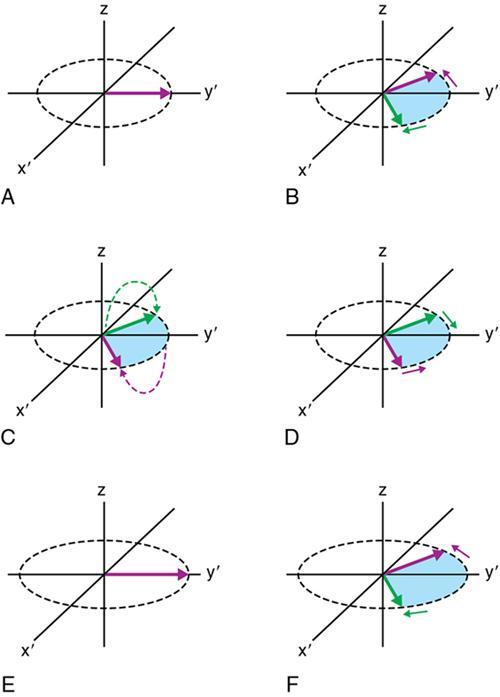
FID and creating echoes
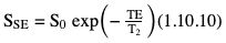
Spin-echo approach
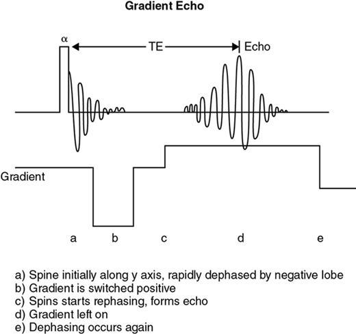
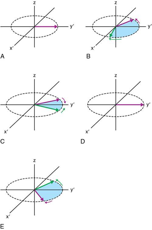
Gradient-echo approach
Relaxation time parameters (TE and TR)
Fourier transform

Related posts:
![]()
Stay updated, free articles. Join our Telegram channel

Full access? Get Clinical Tree


Radiology Key
Fastest Radiology Insight Engine